Could a variable mass oscillator exhibit the lateral instability?

N. Danilović, M. Kovačević, and V. Babović

The Faculty of Science, Institute of Physics, Kragujevac

Abstract

The paper deals with the physical states of an elastic pendulum near its resonant point. As far as we know, in the reach literature on the subject there is a lack of experimental studies of variable mass harmonic oscillations. We perform a set of such measurements in order to investigate the behavior of non-stationary oscillators including autoparametric resonance conditions. Our experiments reveal that the lateral instability really starts when the bob mass equals the critical value predicted by the linear theory of the phenomenon. The subsequent evolution of the motion is generally very complex and strongly depends on many subtle details of the physical system at the early moments in the post-resonant period.

We also undertook the detailed computational job to compare the full theory of the elastic pendulum with the linear approximation and found that the main predictions of the linear theory, as stated in [1], are correct. The characteristic comparisons of vertical and horizontal oscillations are presented.

1. Introduction

The elastic pendulum (also known as the extensible pendulum or spring pendulum) is a simple pendulum with a spring incorporated in its string. This sort of harmonic oscillator placed in a gravitational field sometimes exhibits loss of lateral stability. The horizontal or pendulum oscillations of such kind are due to parametric resonance.

As we will describe below, if the pendulum weight is forced to start with some vertical displacement, but no horizontal displacement, vertical oscillations are set up and the bob will simply bounce up and down. However, if the frequency of the vertical harmonic oscillations is exactly twice the pendulum frequency, the vertical motion becomes parametrically unstable. It means that any small initial horizontal deviation of the bob from the vertical equilibrium position results in an exponentially increasing pendulum motion. Evidently, the energy of the spring oscillations goes into the pendulum oscillations. After the full amount of the energy is transferred, the centrifugal force initiates the reverse process. The initial state will be soon restored. Of cause, then begin a novel cycle of this recurrence process, and so on.

The elastic pendulum is seemingly a simple physical system. Nevertheless, it can exhibit very complex phenomena, which require for the satisfactory explanations rather sophisticated analytical methods. Therefore, this mass-spring-sting combination has been treated many times in the past, as a challengeable, nothing but genuine problem. Aničin, Davidović and Babović [1] give a literature survey of the subject, with short critical notes of some extent. In addition, the elastic pendulum has been often used as an efficient model when treating different problems in several fields of physics, e.g. in accelerators physics (theory of orbital oscillations), nonlinear optics and plasma physics (wave-wave interactions).

In the cited paper [1] the authors have presented the linear theory of the elastic pendulum. The standpoint there adopted is the Ince-Strutt stability chart of the Mathieu equation. They have determined graphically the range of mass leading to instability for particular amplitude of the initial vertical oscillation and the corresponding growth coefficient. In the beginning, they have derived the relevant system of two nonlinear coupled differential equations. Further, the authors have restricted their analyses to the case of motion limited to a relatively small region around the origin in the ($x,y$) plane, i.e. for $x\ll 1$ and $y\ll 1$. The linear system of equations appeared fully capable to demonstrate the parametric resonance at $\omega _{2}=2\omega _{1}$ and practically to remove the possibility of the parametric resonance at $\omega _{2}=\omega _{1}$ (here, $\omega _{1}$ and $\omega _{2}$ are, respectively, the angular frequencies of horizontal and vertical harmonic oscillations).

In this paper, we are going to perform two tasks. First, we wish study numerically the original, nonlinear system of coupled differential equations for the given lateral instability problem — without any linearization procedure. So far, a direct numerical analysis has not been performed and it must be curious to now how much the linear approximation is reliable. Secondly, we have done an experiment with variable mass elastic pendulum. Our aim was to study the resonant process while passing during time the critical combinations of relevant parameters. As far as we know, now one yet has reported on such type of observations when dealing with a laterally unstable harmonic oscillator.

In the next section we will, in the sake of readers comfort, present the detailed theory of the elastic pendulum and outline the relevant equation published in several papers on the subject, among them in above cited reference [1].

2. Theory

In order to write down all the necessary expressions, let us take the advantage of the figure 1, where is sketched the elastic pendulum: a bob hanged on string with an incorporated spring.

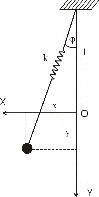
Fig. 1 Elastic pendulum in the position when its string makes the angle $\phi$ with the vertical $Y-$ axis; $\left(x,y\right)$ point defines the instantaneous position of the pendulum weight; the point O is the origin of the Cartesian right-handed system and means the locus of weight in the static equilibrium.

The Cartesian axes $X,Y$ start from the origin that physically means the equilibrium point of the attached weight. The coordinates $\left(x,y\right)$ give the instantaneous position of the weight. We will designate the spring stiffness constant with $k$. For the mass of the bob let us write $m$. This mass depends on time. The angular frequency of the vertical harmonic oscillations is then

$$\omega _{2}=\sqrt{\frac{k}{m}}. \tag{1}$$

Assume $g$ is the acceleration due to gravity. The natural length of the pendulum we will denote with $\ell _{0}$. When the bob is attached, the spring would become longer, according to the relation

$$\ell =\ell _{0}+\ell _{1}. \tag{2}$$

Of cause, the additional length $\ell _{1}$ is determined with the above-defined parameters, and in fact

$$\ell _{1}=\frac{mg}{k} \tag{3}$$

In the operating position depicted on the figure, the bob is for the distance $\lambda$ apart from the point of suspension (therefore, $\lambda$ is the pendulum length at a given instant). The Cartesian coordinates of the bob in this position are $x$ and $y$, whereas the polar ones are $\lambda$ and $\phi$.

Using the geometry (sketched on the figure 2) of the two forces which are

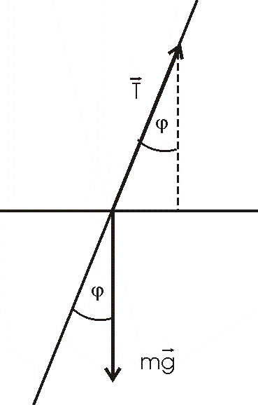
Fig. 2 Forces acting on the pendulum bob in the position sketched in Fig. 1; $\vec{T}$ is the string tension, $\vec{g}$ the acceleration due to gravity;

acting on the oscillating bob, we write according to the Newton second law

$$m\vec{a}=\vec{T}+m\vec{g}. \tag{4}$$

The projection of this vector equation on the axis of abscissas yields

$$m\frac{d^{2}x}{dt^{2}}=-T\sin \phi. \tag{5}$$

Here we may put $\sin \phi =x/\lambda$. The force in string, according to Hook’s law reads

$$T=k\left(\lambda -\ell _{0}\right). \tag{6}$$

Hence, we obtain

$$m\frac{d^{2}x}{dt^{2}}=-k\left(\lambda -\ell +\ell -\ell _{0}\right)\frac{x}{\lambda }. \tag{7}$$

Recall that $k\left(\ell -\ell _{0}\right)=mg$. The above equation could be divided with the length $\ell$; in what follows we shell consider that $x$ and $\lambda$ are the normalized quantities. Therefore,

$$\frac{d^{2}x}{dt^{2}}=-\frac{k}{m}\left(\lambda -1\right)\frac{x}{\lambda }-\frac{g}{\ell }\frac{x}{\lambda }. \tag{8}$$

We can extent the both sides of this equation with the expression $\omega _{1}^{2}x$, where $\omega _{1}=\sqrt{g/\ell }$. The equation which originate from such a procedure could be put in the form

$$\frac{d^{2}x}{dt^{2}}+\omega _{1}^{2}x=-\left(\omega _{2}^{2}-\omega _{1}^{2}\right)\frac{\lambda -1}{\lambda }x. \tag{9}$$

Using the abbreviation

$$\beta =\omega _{2}^{2}-\omega _{1}^{2}, \tag{10}$$

we arrive at the expression

$$\frac{d^{2}x}{dt^{2}}+\omega _{1}^{2}x=-\beta x\frac{\lambda -1}{\lambda }. \tag{11}$$

Now we shell seek what would be the $y$-component of the vector equation (4). First, we have

$$m\frac{d^{2}y}{dt^{2}}=-k\left(\lambda -\ell _{0}\right)\cos \phi +mg. \tag{12}$$

The extension used above in the equation (8) gives now once more from (11)

$$m\frac{d^{2}y}{dt^{2}}=-k\left(\lambda -1\right)\cos \phi +mg\left(1-\cos \phi \right). \tag{13}$$

Also, we shell incorporate here our familiar quantities $\omega _{1}$, $\omega _{2}$ and $\beta$. Therefore, we arrive at

$$\frac{d^{2}y}{dt^{2}}+\omega _{2}^{2}y=-\beta +\beta \frac{1+y}{\lambda }. \tag{14}$$

We have obtained the two necessary equations. As an intermediate résumé, let us group here these equations, (11) and (14), calling them now the equations (I) and (II):

$$\frac{d^{2}x}{dt^{2}}+\omega _{1}^{2}x=-\beta x\frac{\lambda -1}{\lambda }, \tag{I}$$ $$\frac{d^{2}y}{dt^{2}}+\omega _{2}^{2}y=-\beta +\beta \frac{1+y}{\lambda }. \tag{II}$$

The possible linearization process assumes the validity of approximations $x\ll 1$ and $y\ll 1$. It leads to the approximated equation pair (see the Appendix A)

$\frac{d^{2}x}{dt^{2}}+\omega _{1}^{2}x=-\beta xy$, (I-$\ell$)

$\frac{d^{2}y}{dt^{2}}+\omega _{2}^{2}y=-\frac{1}{2}\beta x^{2}$, (II-$\ell$)

which were the basis for the linear analysis conducted in [1]. As we have already pointed out, we shell here numerically treat the original pair of coupled equations (I) and (II), in its full nonlinear content. Nevertheless, because it would be useful in our subsequent analysis of experimental data, we shell now in short repeat the basic conclusions of the linear theory.

Suppose we start the vertical simple harmonic oscillation

$$y=A\cos \left(\omega _{2}t\right) \tag{15}$$

of some amplitude $A$. Therefore, we have from (I-$\ell$)

$$\frac{d^{2}x}{dt^{2}}+\omega _{1}^{2}x=-\beta xA\cos \left(\omega _{2}t\right). \tag{16}$$

Consequently, the differential equation

$$\frac{d^{2}x}{dt^{2}}+\left[\omega _{1}^{2}+\beta A\cos \left(\omega _{2}t\right)\right]x=0 \tag{17}$$

has to be compare with the well-known Mathieu equation [6] in its standard form

$$\frac{d^{2}x}{d\tau ^{2}}+\left[a+16q\cos \left(2\tau \right)\right]x=0. \tag{18}$$

We conclude that the parameters satisfy these relations:

$$\tau =\frac{1}{2}\omega _{2}t, \tag{19}$$ $$a=4\frac{\ell _{1}}{\ell }=4\frac{mg}{k\ell }, \tag{20}$$ $$q=\frac{A}{4}\left(1-\frac{a}{4}\right). \tag{21}$$

The condition $a=1$ corresponds to the parametric resonance $\omega _{2}=2\omega _{1}$. This condition acts when we have $4m_{R}g=k\ell$, or

$$m_{\text{R}}=\frac{k\ell _{0}}{3g}. \tag{22}$$

Therefore, the formula (22) specifies the resonant mass. By this value of mass, the system spring-mass quickly develops the lateral instability.

From the very definition of the spring stiffness constant $k$ we may write

$$k=\frac{\Delta m\;g}{\Delta \ell }. \tag{23}$$

After putting this value into the result (22), we obtain immediately $m_{\text{R}}=\frac{1}{3}\Delta m\frac{\ell _{0}}{\Delta \ell }$. If $M_{\text{D}}\equiv \Delta m$ is those mass which would double the natural length of spring, $\ell _{0}$, a simple and retentive formula arises:

$$m_{\text{R}}=\frac{M_{\text{D}}}{3}. \tag{24}$$

Finally, we would like to remark what follows. In some applications using the latest version of the Mathematica computational system we found appropriate the solutions of the form

$$\frac{d^{2}x}{dt^{2}}=-\omega _{\text{v}}^{2}\frac{1}{p}\frac{\lambda -\ell _{0}}{\lambda }x, \tag{25}$$ $$\frac{d^{2}y}{dt^{2}}=-\omega _{\text{v}}^{2}\frac{1}{p}\frac{\left(\lambda -\ell _{0}\right)\left(\ell +y\right)}{\lambda }+g, \tag{26}$$

instead of (I) and (II). The dimensionless parameter $p$, when passing through unity, defines the nonlinear coupling resonance condition. The derivation of the above equations is straightforward and we omit here the proof.

3. Computations

As it already has been announced, we shell now numerically treat the set of two nonlinearly coupled equations (I) and (II). The figure 3 shows the time evolution of the elastic pendulum motion when the conditions of the autoparametric resonance are nearly or fully satisfied. Here our choice of parameters was: the spring stiffness constant 100 N/m and the equilibrium length of string/spring combination 100 cm.

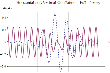
Fig. 3 Mathematica 6.0 plot of the full nonlinear system of equations (I), (II); time evolution of the vertical oscillations (continuous line) and horizontal oscillations (dashed line); $k=50$ N/m, $\ell =1$ m, $m=m_{\text{R}}=1.274$ kg.

In fact, we have presented two curves on the same plot. The vertical oscillations start with a given amplitude. The initial horizontal displacement is very small, but cannot be put to zero. After some periods of oscillations, a considerable amount of energy of this mode is transferred to the horizontal, or pendulum mode of oscillations. The amplitude of the pendulum mode exponentially grows. At some instant, designated on the graphic with the tick 8, almost all the energy is in this horizontal mode of motion; simultaneously, the amplitude of vertical oscillations is at their minimum. The process is now reversed. There are two cycles of vertical oscillations in each pendulum period. Physically, the centrifugal force acts as an excitation term to the vertical oscillations. Soon the initial state is restored. The oscillating energy is uninterruptedly flowing from the vertical motion into the horizontal motion and vice versa.

The linear theory, under the same condition valid for the figure 3, gives the result we plotted in the figure 4.

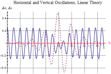
Fig. 4 Mathematica 6.0 plot of the linearized system of equations ($I-\ell$), ($II-\ell$); time evolution of the vertical oscillations (continuous line) and horizontal oscillations (dashed line); $k=50$ N/m, $\ell =1$ m, $m=m_{\text{R}}=1.274$ kg.

Let us now examine the figure 5. There we have plotted the horizontal component of the above collective graphic and added the horizontal curve obtained according to the approximated pair of equations (I-$\ell$) and (II-$\ell$).

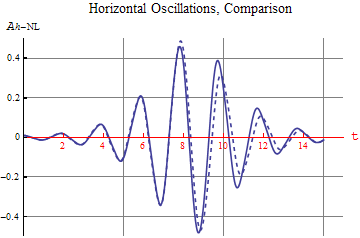
Fig. 5 The comparison of solutions for horizontal oscillations; exact theory (continuous line) and linear theory (dashed line); $k=50$ N/m, $\ell =1$ m, $m=m_{\text{R}}=1.274$ kg.

The dashed line corresponds to linear solution. The difference between the solutions seems to be hardly discernible. Evidently, the linearization has in this case its full justification, because it spreads analytical possibilities in the problem treated.

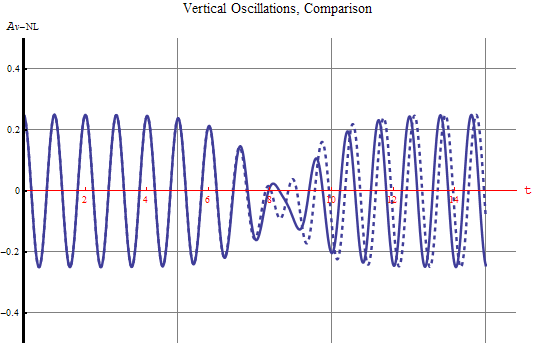
Fig. 6 The comparison of solutions for vertical oscillations; exact theory (continuous line) and linear theory (dashed line); $k=50$ N/m, $\ell =1$ m, $m=m_{\text{R}}=1.274$ kg.

Finally, let us see in the figure 6 the comparison of the two solutions concerning the vertical oscillations. The dashed curve is the linear solution. Again, we have the good agreement between the exact and approximated formulae.

4. Apparatus

We must begin the experimental work performing two preliminary measurements: a) the determination of the spring stiffness constant, and b) the determination of the string length. The both tasks must be done as carefully as possible, because the reliability of the results depends on it.

Determination of the spring stiffness constant In fact, this procedure is standard and could be easily performed applying Hook’s law $k=\frac{\Delta m\,g}{\Delta \ell }$. Nevertheless, one must be cautious. The spring will not stretch at all under the action of a small gravitational force $\Delta m\,g$. The measurements are to be performed well in the region of full linearity, sufficiently above the critical force. We did so, applying seven masses, one by one, in the range from 20 g to 80 g. Each time we have readout the corresponding lengthening of the spring. The pairs of such measured values were indicated into a graphic. Through the set of points we have plot a strait line by means of the least squares method.

The spring we finally choose as appropriate for our measurements was proved, according to this procedure, to have the stiffness constant $k=9.2$ N/m.

Determination of the natural pendulum length In our notation, $\ell _{0}$ is the distance, with no weight attached, from the hook where the spring is attached to its other end. We found this length was nearly 11 cm. To this value must be added, as we have estimated, additional 4 cm (2 cm from the hook on the vessel to the center of mass of the vessel containing water and 2cm for two small peaces of string on both sides of spring). The vessel is the plastic cylinder with diameter 6 cm and height 4.5 cm. It could optimally contain 100 g of water.

The effective length of the spring with no mass attached, i.e. the natural length of the pendulum was so determined to be $\ell _{0}=15$ cm.

Determination of the spring mass The mass of our spring is $m_{\text{spring}}=12.75$ g. The mass of the empty vessel is $m_{\text{tank}}=19.5$ g. The bob mass of the elastic pendulum in action is the sum $m=m_{\text{tank}}+m_{\text{water}}$. We see that nearly is satisfied $m_{\text{spring}}\ll m$.

In our theory, the mass of the spring is regarded as negligible.

5. Experiment

We made in the center on the bottom of the vessel a small cyclic opening 1mm in diameter. On the top side of the vessel, there is a hole for the inlet of air while the water leaks out through the opening. We proofed, in non-oscillating state, the initially full of water vessel would be empty in nearly 25 second. Making our variable mass oscillator, we were fully aware of experimental troubles, which could follow the usage of a fluid-weight changing in time, even if in a controlled manner (Flores, Solovey & Gil, 2003b).

We excite a periodic oscillation of the type $y=A\cos \left(\omega _{2}t\right)$ by pulling down the weight and setting it free with the zero velocity at $t=0$. As the oscillations go, the mass of the weight diminishes and the motion of vessel becomes quicker. At some instant, the pendulum starts to develop the horizontal oscillations. The instability grows fast and soon we see only the pendulum mode of motion. We have taken a set of photographs of this phenomenon and one of these is shown on the picture.

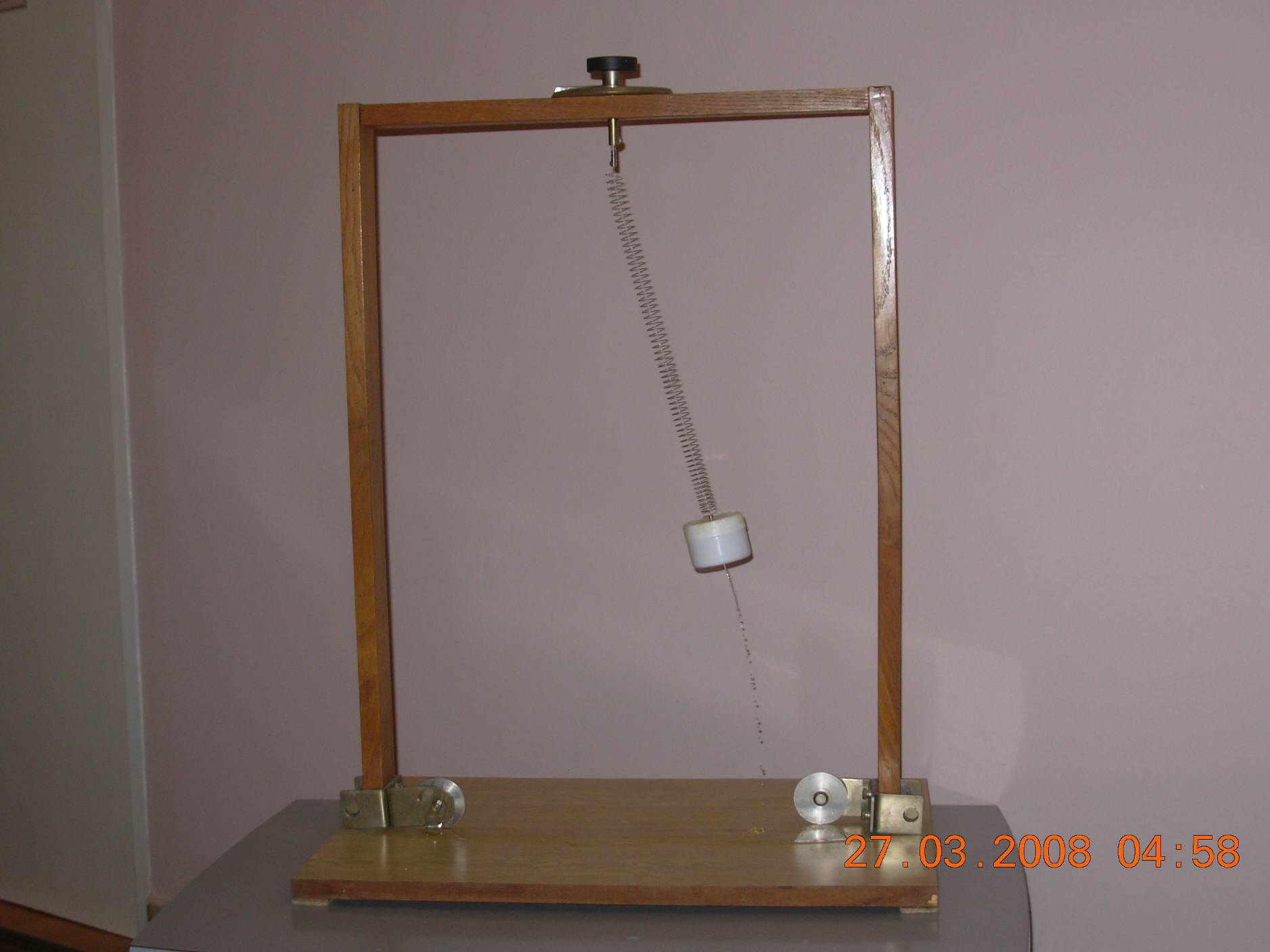
Photograph of the apparatus in action; the instant of maximum horizontal deviation; the flow of water is visible; in this pendulum mode of oscillations, the flow rate depends on the water height in vessel, but otherwise is constant.

Obviously, the oscillator goes through the point of its parametric resonance. We have measured the corresponding critical mass of weight (the mass of vessel with the mass of remaining water) in a series of observations.

The mean measured critical mass was found to be $m_{\text{R}}^{\text{m}}=48.25$ g.

Now we shell compute the theoretical critical mass. Using the above-mentioned values for the free pendulum length and the spring stiffness constant we obtain $m_{\text{R}}^{\text{t}}=\frac{k\ell _{0}}{3g}=46.89$ g.

The percent error is $\delta =2.8$ %.

At this point, we have undertaken a computational simulation of the phenomenon. We have modeled the process of water leaking down adopting the linear mass dependence of time, $\frac{m}{m_{\text{R}}}=C_{1}\left(1-C_{2}t\right)$. In the literature, one can find the evidence that sand sifts very nearly at constant rate (Flores, Solovey & Gil (2003a)). For water, this is only but an approximation (certainly, there are laboratory techniques, which would help to overcome the trouble [5]). From a vertically oscillating vessel, the flow rate also oscillates. (We plan to study particularly this phenomenon in a separate paper.) Nevertheless, near the resonant point we shell try with the indicated linearization. Assuming the pair of coupled equations is sufficiently true in the case of a variable mass, we have looked for the solution in the Mathematica 6.0 program. The results are shown on Figs. 7-9.

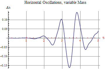
Fig. 7 The time evolution of the horizontal oscillations according to nonlinear theory; parameters used in experiments: $k=9.2$ N/m, $\ell _{0}=0.15$ cm, $C_{1}=1.3$, $C_{2}=0.02$; $m_{\text{R}}=0.0467$ kg; $m=m_{\text{R}}C_{1}\left(1-C_{2}t\right)$.

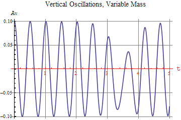
Fig. 8 The time evolution of the vertical oscillations according to nonlinear theory; parameters used in experiments: $k=9.2$ N/m, $\ell _{0}=0.15$ cm, $C_{1}=1.3$, $C_{2}=0.02$; $m_{\text{R}}=0.0467$ kg; $m=m_{\text{R}}C_{1}\left(1-C_{2}t\right)$.

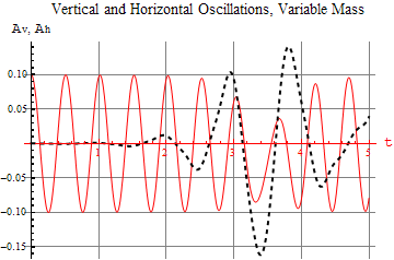
Fig. 9 The comparison of oscillations; vertical oscillations (continuous line), horizontal oscillations (dashed line); parameters used in experiments: $k=9.2$ N/m, $\ell _{0}=0.15$ cm, $C_{1}=1.3$, $C_{2}=0.02$; $m_{\text{R}}=0.0467$ kg; $m=m_{\text{R}}C_{1}\left(1-C_{2}t\right)$.

Again, we have the excellent global agreement in the frame of our physical model. The process of the lateral instability development wholly coincides with the growth of the pendulum amplitude as well as with the vertical amplitude diminishment. However, let us see the Fig. 10.

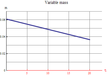
Fig. 10 The pendulum weight is supposed to decrease linearly with time; $m=m_{\text{R}}C_{1}\left(1-C_{2}t\right)$, $m_{\text{R}}=0.0467$ kg; $C_{1}=1.3$, $C_{2}=0.02$;

This figure gives the variable mass versus time. The dependence is of the type $m\left(t\right)=m_{\text{R}}f\left(t\right)$, where $f\left(t\right)=C_{1}\left(1-C_{2}t\right)$ and the resonant mass $m_{\text{R}}=k\ell _{0}/\left(3g\right)$. The constants are $1.3$ and $0.02$, respectively. We already know that the resonant mass corresponding to the in measurements adopted parameters amounts to but a little 49 grams. From Fig. 7 we read that the maximum lateral weight deviation occurs 3.5 seconds after the motion started. From Fig. 10 we may conclude that for $t=3.5$ s the mass is $m\approx 55$ g. The computed mass value, obviously, do not coincides very well with the measured mass value. However, the error of about $13\%$ could not be regarded as quite unsatisfactory.

Factors, which supposedly could cause the discrepancy, are numerous; the main, as we believe, is the rude and incomplete model of the vessel with leaking water. In addition, the physicists in this area of experimental physics well know it is extremely important to set up the system as precisely as possible — a small error can have a large negative effect on the quality of the results. Concretely, a carelessly started process of the vertical oscillations could initiate an undesired evolution of motion. There are two types of qualitative motion of the elastic pendulum. These are a) crescent and b) lemon oscillations (Rusbridge (1980); Davidović, Aničin & Babović (1996)). None of the both is of primary interest in the current paper; we are amidst the job of searching how the variable mass could affect the motion of an elastic pendulum in connection with the autoparametric resonance: in other words, could the variable mass elastic pendulum demonstrate unstable motion.

As we see, it can and, besides, would help deeper insights into this complex physical phenomenon.

6. Conclusion

This paper deals with the variable mass elastic pendulum. We proved it exhibits the lateral instability, and really under the conditions known to be valid in stationary experiments. When passing through the resonant mass, the strong autoparametric resonance in the system is evident.

While preparing the apparatus, we experimented with many and many strings seeking the optimal combination of string parameters (stiffness constant, length, diameter, mass and so on). Our impression is that the strings of about $k=10$ N/m and $\ell _{0}=10$ cm are preferable, at least in preliminary experiments. Leaking fluids, presumable water, are attractive in designing the variable weights, but we do not exclude other possibilities (first of all, fine sorts of sands offer interesting possibilities). We must be aware that the fluid jet streaming from an oscillating vessel gives a flow rate far from being a constant one. This is a problem deserving its own right.

The non-linear coupled equations (I, II) explain the various curious details in experiments with the elastic pendula very well. Our analyses and computations show that the linearized equations retained the basic capability of the standard elastic pendulum theory; this is important because the simplified equations enable the reach area of analytical activity.

In the paper [4], the authors investigated the problem of the variable mass oscillator rather thoroughly. However, they have not commented at all the possibility that the oscillator passes the region of the lateral instability connected with the autoparametric instability, although their pendulum is evidently elastic (extensible). Our experience is that the variable mass harmonic oscillator can exhibit the lateral instability and this aspect of the problem can not be disregarded.

References

[1] Aničin B A, Davidović D M, and Babović V M, On the linear theory of the elastic pendulum, Eur. J. Phys. 14(1993) 132-135.

The Physics Department of The University of Maryland included this article into Demonstrations Reference File as ‘good article on the elastic pendulum.’

[2] Davidović D M, Aničin B A, Babović V M, The libration limits of the elastic pendulum, American Journal of Physics, 64(3), March 1996.

[3] Flores J, Solovey S, Gil S, Flow of sands and a variable mass Atwood machine, Am. J. Phys. 71 (7), July 2003a, p. 715.

[4] Flores J, Solovey S, Gil S, Variable mass oscillator, Am. J. Phys. 71 (7), July 2003b, p. 721.

The authors remark: “For fluids, the time rate of the mass discharged through an orifice depends on the height of the column and thus is time dependent. In contrast, we show that the flow rate of sand is constant in time and does not depend on its height.” However, we decided to carry out this series of experiments with fluids (water), and postpone the use of sand for a future experimental activity. In addition, what is most important for us, the authors proved “that $\omega$ was well described by the relation $\omega ^{2}=k/m\left(t\right)$.”

[5] Mariotte’s vessel keeps the escape velocity constant. The vessel has a hole in the wall of a Heron Ball (or similar vessel). The hole is below the lower end of the tube. In addition, the discharge velocity could be kept constant by various siphon arrangements.

[6] McLachlan N W, Theory and Application of Mathieu Functions, Oxford: Clarendon, 1947.

[7] Rusbridge M G, Motion of the Spring Pendulum, Am. J. Phys. 48, (1980), p. 146.

Appendix A

The linearization of the coupled equations of the elastic pendulum

Let us see first the equation (I).

$$\frac{d^{2}x}{dt^{2}}+\omega _{1}^{2}x=-\beta x\frac{\lambda -1}{\lambda }. \tag{I}$$

We need to approximate the rhs expression:

$-\beta x\frac{\lambda -1}{\lambda }\to -\beta x\frac{\sqrt{\left(1+y\right)^{2}+o^{2}}-1}{\sqrt{\left(1+o\right)^{2}+o^{2}}}$. (A-1)

It means

$-\beta x\frac{\lambda -1}{\lambda }\to -\beta xy$, (A-2)

in agreement with the equation (I-$\ell$) which reads

$\frac{d^{2}x}{dt^{2}}+\omega _{1}^{2}x=-\beta xy$. (I-$\ell$)

Let us now focus our attention on the second equation (II)

$$\frac{d^{2}y}{dt^{2}}+\omega _{2}^{2}y=-\beta +\beta \frac{1+y}{\lambda }. \tag{II}$$

The rhs converges to

$-\beta +\beta \frac{1+y}{\lambda }\to -\beta +\beta \frac{1+y}{\sqrt{\left(1+y\right)^{2}\left[1+\frac{x^{2}}{\left(1+y\right)^{2}}\right]}}$, (A-3)

$\to -\beta +\beta \frac{1+y}{1+y}\frac{1}{1+0.5\frac{x^{2}}{\left(1+o\right)^{2}}}$, (A-4)

$\to -\beta +\beta \left(1-\frac{1}{2}x^{2}\right)$, (A-5)

$\to -\frac{1}{2}\beta x^{2}$. (A-6)

This is in agreement with the equation (II-$\ell$):

$\frac{d^{2}y}{dt^{2}}+\omega _{2}^{2}y=-\frac{1}{2}\beta x^{2}$. (II-$\ell$)

The linear set of the two equations, which we have just derived applying the reasonable approximations to the original equations of the elastic pendulum are easy adaptable to the forms rightly required by the Mathieu equation.

Appendix B

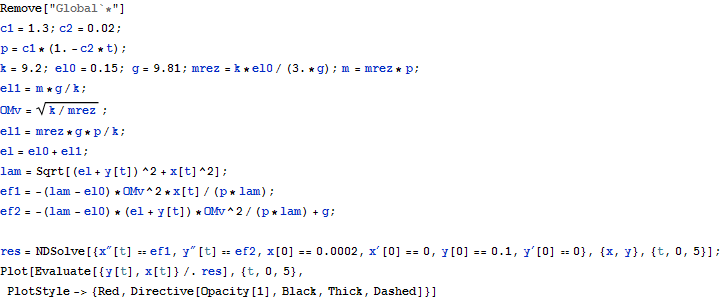
The listing of the Mathematica 5.0 programme used in the Experiment section

Sažetak

Ovaj se rad bavi fizičkim stanjima elastičnog klatna u blizini rezonantne taške. Koliko znamo, u bogatoj literaturi koja se tiče obe problematike malo je eksperimentalnih radova posvećenih harmonijskom oscilovanju s promenljivom masom. Organizovali smo niz takvih merenja s ciljem istraživanja ponašanja nestacionarnih oscilatora u zoni autoparametraske rezonancije. Naši eksperimenti otkrivaju da bočna nestabilnost zaista počinje kad je masa tega jednaka kritičnoj vrednosti koju predviđa linearna teorija pojave. Potonja evolucija kretanja uopšte je vrlo složena i jako zavisi od mnogih detalja fizičkog sistema u početnim momentima post-rezonantnog perioda.

Takođe smo preduzeli mnoga izračunavanja da uporedimo punu teoriju elastičnog klatna sa linearizovanim jednačinama; potvrdili smo predikcije linearne teorije, koje su ustanovljene u radu [1].