The Sun lightens and enlightens: high noon shadow measurements

Vukota Babović and Miloš Babović

Department of Mathematics, Physics and Informatics,

The State University of Novi Pazar, Vuka Karadžića bb,

36300 Novi Pazar, Serbia

Abstract

Being aware of the fact that some contemporary physicists and science experts include the Eratosthenes’ measuring of the Earth’s circumference in the most beautiful experiments in physic ever performed, we have revisited this famous event from the history of science. It turns out that some interesting generalizations are possible. We found a new formula, entirely eratosthenian in spirit, for a planet year duration. We believe that the great Alexandrian sage can play a greater role in university courses of physics, at least in those which treat environmental problems.

1. Introduction

There are several examples of advanced knowledge which arrived to us from the old times, mainly from the ancient Greeks. For example, the works of Archimedes, Aristarchus, Democritus, and Euclid stood the test of time and may look to us as magnificent proofs of the power of the human common sense. The journal Physics World rose at the beginning of the third millennium an interesting question: what could be the most beautiful physical experiment ever performed. A poll was organized among friends and journal’s readers. This searching gave the top ten experiments [1]. The seventh place on that hit list was reserved for Eratosthenes and his method of Earth’s circumference measurement. So, this prodigious person of the pre-Christian era found himself in the exclusive scientific society, together with giants such as Newton, Young or Rutherford. It is not likely that any physicist could deny the exceptive effectiveness of Eratosthenian reasoning and proceeding.

Eratosthenes was the first person to succeed in estimation of Earth’s size. At the same time, as far as we know, he did it quite precisely, although this fact is not of the prime importance. For the sake of reader’s convenience, we shall now briefly rephrase the key points of Eratosthenes’ measurement.

In the city of Syene (now Aswan in Egypt), the story tells, was at Eratosthenes’ era a deep well. This well was peculiar and widely known because its bottom was insolated by the sun rays, but only during one day in the year and only at local noon of that day, which appeared to be the event of summer solstice. Being in Alexandria (which lies approximately on the north from Syene) as the chief librarian of the famous Royal Library of Alexandria at its finest times, Eratosthenes read a story about that well and, at the very solstice, made the most of the clear sky and measured the length of a horizontal shadow casted by a vertical opaque rod. It was enough to calculate the Sun’s angle of elevation at local noon on the solstice day in Alexandria: 7°12’ south of the zenith. Therefore Eratosthenes concluded that the Earth’s circumference ($C_{\text{E}}$) divided by the distance from Alexandria to Syene ($d_{\text{AS}}$) must be equal to $360^{\circ}/7^{\circ}12'\approx 50$. So the formula $C_{\text{E}}=50d_{\text{AS}}$ should give the true circumference, once the distance was known. The legend also says that Eratosthenes managed to infer the distance data, and we have no remark against his numerical result (25 000 stadia. This ancient unit is defined as 166.7 meters [2]). The facts which we praise so high are his faith not in written words but in the scientific method (Nullus in verba, as the British Astronomical Society logo says) and his transparent physical model, so boldly manifested through the measuring procedure.

It is sometimes useful to see: what is the valuable knowledge in a heap of facts, often a bit mythically interconnected, which yields for a very long period of time to some, not always truly credible, notorious story. A lots of impertinent details are to be thrown off. We recently tried in the Journal to treat in this way two of several possible themes [3], [4]. Maybe, this paper is another example of the sort.

Now we are going to present our measurements, most of them of noon shadow length generated by gnomons or triangle-type objects. The obtained data will be compared to the theoretical values that follow the simple model of the daily Earth’s insolation. As we shall see, the model is approximate, but quite useful in many applications. First of all, we succeeded in deriving an expression for the duration of the Earth’s year. As far as we know this formula is a novel result. Also, we have experimentally tested predictions of our theory, fully in the eratosthenian spirit, and found the good agreement, as we shall later see in detail.

2. Sun angle measurement methods

The moments of sunrise and sunset, the momentary position of the Sun on the sky, as well as the duration of daylight are important events in our everyday life. All of these are directly related to the length of the shadow of a vertical opaque stick (gnomon), thrown on a horizontal flat surface. Using tehnology, these measurements are possible in some very witty and unexpected ways [5]. Here, we are interested in simplest possible tools. A handy gnomon helps in doing preliminary jobs in many scientific, engineering and educational projects. It can be realized in a variety of ways, and we preferred a simple setup with a camera tripod, shown on figure 1.

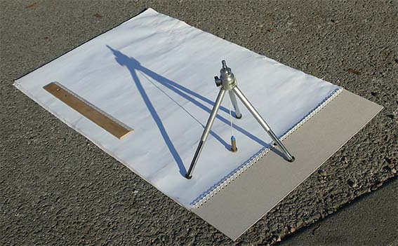
Figure 1. Tripod-type gnomon

A small weight, fastened by a string to the central elevated point of this tripod, gives the vertical line by any position of legs. We have used this simple setup for various relevant shadow length measurements, but mostly for monitoring the tilt angle of incident sun rays during the diurnal apparent moving of the Sun over the sky.

And yet, we performed shadow measurements at local noon with great comfort and (as we shall see later) surprisingly high accuracy by even simpler equipment: an ordinary right triangle.

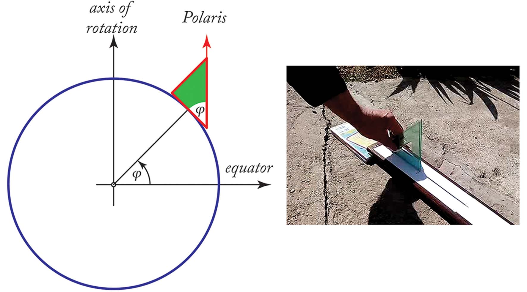
Figure 2. Right $\varphi -$ triangle

The best of such triangles are those who have another angle equal to the latitude of the location of the measurement (right $\varphi -$ triangle). As shown on figure 2, we may hold such triangle with opposite side vertical and the adjacent side horizontal; as a result, the hypotenuse shall point toward the North Star (Polaris)¹.

Of course, Polaris is not to be seen at the noon. Nevertheless, the shadow of the triangle stretches itself exactly toward the Nord and at the same time its width is minimal. Also, in this configuration we can register two shadows (of the opposite side and of the hypotenuse), which means that our angle-teller now immediately delivers a twofold result (we shall discuss this further in Section 6).

3. Model of the Earth’s insolation

We shall now seek for the main equation which governs the Earth’s illumination by the Sun. The situation we treat is shown on Figure 3. (The inspiration for ideas in this Section we found in a fine popular book [6]).

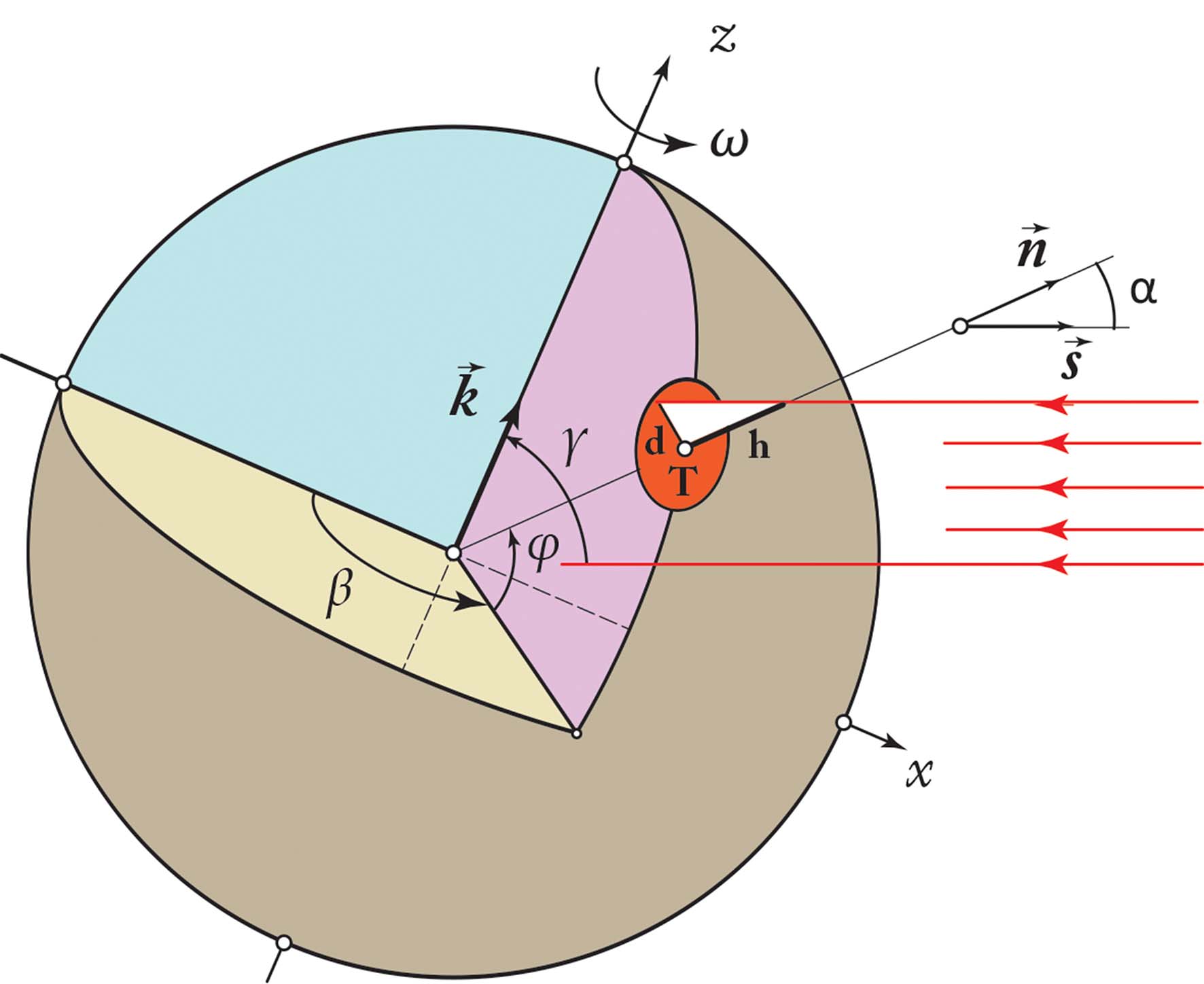
Figure 3. Small horizontal platform upon Earth in morning hours of a clear day

At the point P on the Earth a rod of the height $h$ is vertically stuck into the ground and it casts a shadow of the length $d$ on a horizontal plane. This length as well as its direction varies during a day because of the diurnal rotation of the Earth about the $z$ axis.

The coordinate system shown on figure 3 is the right-handed Cartesian system, with its origin placed at the center of the Earth. The fundamental plane is the equatorial plane. The primary direction with its x-axis is toward the high noon point; the y-axis is $90^{\text{o}}$ to the east in the fundamental plane. The $z$ axis is perpendicular to the fundamental plane and points toward the North Pole.

We designated as $\vec{s}$ the unit vector in the direction Earth — Sun. Also, let $\vec{n}$ be the unit vector in the direction of the rod. As we have plotted, the angle $\alpha$ is defined by these two directions and we shall refer to it as the sun angle. The quantity $\omega$ stands for the angular velocity of the Earth’s rotation around the z-axes. (Note that figure 3 refers to the time moment $t=\beta /\omega$, where $\beta$ is the corresponding hour angle — at the midnight at Greenwich position $\beta =0$). Further, let $\vec{k}$ be the unit vector in the direction of the $z$-axis. The angle between z-axes and sun rays we marked as $\gamma$; we shall determine this angle later, for a given latitude and a day of the year.

The projections of the unit vector $\vec{s}$ on the axes of the described coordinate system are:

$$\vec{s}=\left[\sin \gamma ,0,\cos \gamma \right] \tag{1}$$

The projections of the unit vector $\vec{n}$ on the axes of the same system of axes are

$$\vec{n}=\left[-\cos \varphi \cos \omega t,-\cos \varphi \sin \omega t,\sin \varphi \right] \tag{2}$$

The dot product of these two unit vectors now gives the cosine of the sun angle

$$\cos \alpha =\vec{n}\cdot \vec{s}=\cos \gamma \sin \varphi -\sin \gamma \cos \varphi \cos \beta \tag{3}$$

The angles $\varphi$ and $\beta$ are, naturally, given quantities, defined by the location of the point P and the time during a day.

Now it is necessary to find the unknown angle $\gamma$.

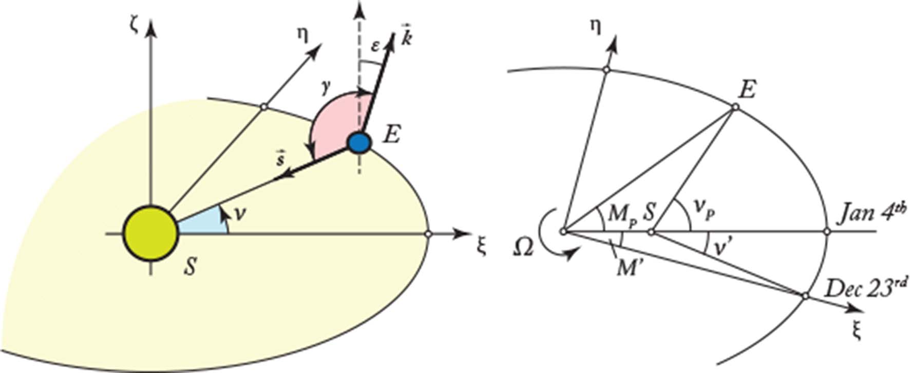
Figure 4. Transient position of the Earth on her orbit around the Sun

Figure 4 left shows the Earth on its orbit around the Sun and the right-handed rectangular heliocentric ecliptic coordinate system: the origin is the center of the Sun, the plane of the ecliptic is the fundamental plane, the $\xi$ axis (the primary direction) points toward the moment of the winter solstice (therefore we shall refer to it as the solstice coordinate system), the $\eta$ axis is $90^{0}$ to the east in the fundamental plane, and the $\zeta$ axis is perpendicular to the plane and points toward the north ecliptic pole.

The angle $\gamma$ can be determined as a function of the two others, $\varepsilon$ and $\nu$. The first is the Earth’s tilt (the angle between the ecliptic and the celestial equator on the celestial sphere; or between the axes $z$ and $\zeta$): the second is the true anomaly (the angular parameter that defines the position of the Earth during its elliptical path around the Sun; the angle between the direction of periapsis and the current position of the Earth, as seen from the main focus of the ellipse) corrected by the angle between Sun-Earth’s winter solstice direction and Sun-Earth’s perihelion direction.

Three components of the unit vector $\vec{s}$ in this $\left(\xi ,\eta ,\zeta \right)$ system are

$$\vec{s}=\left[-\cos \nu ,-\sin \nu ,0\right] \tag{4}$$

Further, three components of the unit vector $\vec{k}$ are

$$\vec{k}=\left[\sin \varepsilon ,0,\cos \varepsilon \right] \tag{5}$$

The dot product of these two unit vectors gives $\cos \gamma$ by definition:

$$\vec{s}\cdot \vec{k}=\cos \gamma =-\sin \varepsilon \cos \nu. \tag{6}$$

Let us remark that in the first approximation (the uniform rotation of a body on a cyclic orbit) we would have in (6) the mean anomaly [7]

$$M=\Omega \tau \tag{7}$$

instead of the parameter $\nu$. Often we measure and compute the angular velocity $\Omega$ in practical units (degrees per day), consequently the time $\tau$ is the number of days from the beginning of the year².

4. Equations of insolation

In the right-handed rectangular coordinate system based on the ellipsis axes, figure 4 right (we shall refer to it as the perihelion coordinate system) where angles are measured counterclockwise, starting from the major axis (in another words, from the Sun-Earth’s perihelion direction) the difference between the true anomaly and the mean anomaly is regularly termed in books on the celestial mechanic as the equation of center [8]. So this quantity has much to do with the ellipticity of the Earth’s orbit. One could commonsensible accept that the difference is practically negligible in points of the two solstices, but perceptible in points of the two equinoxes. If the eccentricity $e$ of the orbit is sufficiently small (the fact we often meet among planets in the Sun’s system) the equation of center follows the series

$$\nu _{P}-M_{P}=\left(2e-\frac{1}{4}e^{3}\right)\sin M_{P}+\frac{5}{4}e^{2}\sin 2M_{P}+... \tag{8}$$

For the eccentricity of the Earth we can accept the value $e=0.0167$[9, p. 121], so terms proportional to $e^{2}$ and higher can be ignored.

During our epoch, the Earth reaches the winter solstice on December 23^rd^, and the perihelion on January 4^th^ ($\Delta \tau =13\;\text{days}$). That’s why we can say that the solstice coordinate system is rotated clockwise by the value $M'=\Omega \Delta \tau$ relative to the perihelion coordinate system. Therefore, in the solstice coordinate system initial value of the true anomaly is not zero, but $\nu '=\Omega \Delta \tau +2e\sin \left(\Omega \Delta \tau \right)$, because it is equal to the true anomaly on the December 23^rd^ in the perihelion coordinate system.

Hence, for our solstice coordinate system equation of center should be corrected by adding a constant parameter $2e\sin \left(\Omega \Delta \tau \right)$, so the equations which we assume to be sufficient as a theoretical model of our measurement activities with shadows equal

$$\cos \alpha =\sin \varphi \cos \gamma -\cos \varphi \sin \gamma \cos \omega t \tag{9a}$$ $$\cos \gamma =-\sin \varepsilon \cos \left[\Omega \tau +2e\sin \left(\Omega \tau -\Omega \Delta \tau \right)+2e\sin \left(\Omega \Delta \tau \right)\right] \tag{9b}$$

These expressions connect six important angles ($\alpha$, $\gamma$, $\varphi$, $\varepsilon$, $\omega t$ and $\Omega \tau$) and they describe a situation when a nearly punctual body insolates a self-rotating and around-it-orbiting (on a ellipse with a small eccentricity) sphere in its vicinity. Obviously, we have ignored some subtle effects such as the refraction of rays in atmosphere and the finite diameter of the Sun — we leave the search for the extreme precession to professional astronomers. The maximum difference between The Astronomical Almanac data and circular orbit CMB data is 1.07 degrees with an average difference in magnitude of 0.428 degrees [10].

Now we know what should be the expected value of the sun angle $\alpha$(see figure 3) at any moment of the day, during each day of the Eratosthenian year, and for all places on the surface where the Sun rises and sets ($\varphi <\left|\pi /2-\varepsilon \right|$). As the Earth’s citizens, we must use $\varepsilon =23.4^{\circ}$[9, p. 121] (To be sure, Martians would prefer the value $\varepsilon =25.19^{\circ}$[9, p. 246], which wouldn’t considerably modify the equation (9b); alas, the red planet is yet an unsettled land).

5. Testing the sun angle formula

Knowing the main law of the sun angle $\alpha$, one can pass over to study special themes in various fields of sciences, such as environmental physics, earth science, climatology [11]. For example, in the paper [12] the authors comment in details how their mathematical model can give the reliable insights into various important phenomena: passage of the seasons or day duration for different latitudes and seasons. Their recent paper [13] deals, among others topics, with the estimation of daily insolation on the horizontal ground. Here we shall try to elucidate, if possible, some kinematical consequences from the geometrical relations which are included in our mathematical model (9).

First of all, let us see whether the elementary predictions of the model are correct or not. We defined the two angular velocities: $\omega =2\pi /T_{\text{D}}$ and $\Omega =2\pi /T_{\text{Y}}$, where periods of rotations are 24 hours and 365.25 days, respectively. Whatever $\varphi$ could be (with respect to the restriction $\varphi <\left|\pi /2-\varepsilon \right|$), from the condition $\Omega \tau =\pi$ follows the solution $\gamma _{\min }=66.6^{\circ}$ (the minimal value of $\gamma$ in the course of one year); it occurs for $\tau \approx 182$ (June 22^nd^). Also, we get from $\Omega \tau =2\pi$ the solution $\gamma _{\max }=113.^{\text{o}}4$; it occurs at $\tau \approx 365$ (December 22^nd^). The two equinoxes, vernal and autumnal, occur when the condition $\Omega \tau =\pm \pi /2$ ($\gamma =\pm \pi /2$) is satisfied, i.e. at $\tau \approx 89$ (March 21^st^) and $\tau \approx 275$ (September 23^rd^), respectively. We are satisfied with the results; the Earth on its orbital revolution reaches these four characteristic positions on the correct day. Of course, further examinations can be undertaken in direct observations during each clear day of the year and for a given day from the sunrise to the sunset.

But, can we realize in the laboratory a physical model of the two astronomical bodies and “artificially” provoke phenomena we wish to analyze? Such a set-up for detailed testing of the consequences of equations (9) is not an unimaginable task. For example, a good terrestrial globe with a scale of nearly 3:40 million (100 cm in diameter) emerged in a broad laser beam would roughly do the job. A small flat optical sensor could thus measure the insolation at the point on the globe’s surface. What is attractive in this idea is the possibility to watch for evolution of optical quantities in various locations upon the surface, and in addition simulating hours of a given day in the year; for few minute one could proceed from the winter situation to the spring season, and so on.

Naturally, direct terrestrial measurements of the solar irradiance parameters can be performed “in vivo”, usually at ease. We didn’t help us but undertook such an ‘in vivo’ eratosthenian shadow measuring in order to try the validity of the equation (9a). During the sunny day on the December 25^th^ 2013 we measured shadow length evolution with our tripod from figure 1 in Belgrade , Serbia ($\varphi =44.82^{\circ}N$, $\lambda =20.5^{\circ}E$, time zone UTC+1). The data have been taken hourly, starting at 8:00 AM (administrative time); eight points were gathered. The results are given in table 1 and plotted on Figure 5.

[TABLE]

Table 1. Hourly measurements of the sun angle in Belgrade, Serbia on December 25^th^ 2013.

The full line is the theoretical curve for $\cos \alpha$, equation (9 $a$). This curve grows from the sunrise defined by the moment $t_{\text{R}}=\left(1/\omega \right)\arccos \left(\cot \gamma \tan \varphi \right)$, till the noon, then diminishes during the afternoon till the sunset, defined by the moment $t_{\text{S}}=\left(1/\omega \right)\left[\pi -\arccos \left(\cot \gamma \tan \varphi \right)\right]$. The length of this day, and of each day of the year, varies with location upon the Earth. Furthermore, the beginning and the end of the day must be defined. We have accepted the definition according to which the day starts, and ends, when the center of the sun is even with the horizon. Also, the refraction of light through the atmosphere affects the very beginning and the very end of the day, but we neglected this effect. Of course, we have been aware of the corrections of daylight durations known as the equation of time [14]. Finally, the day length is $\Delta t_{\text{L}}=t_{\text{S}}-t_{\text{R}}$. The angle $\alpha$ takes its minimal value at the local noon, i.e. at $t_{\text{N}}=t_{\text{R}}+\Delta t_{\text{L}}/2$.

The area of the region bounded by the graph is small in the winter and large in the summer. Apart from this, the cosine graph, for every clear day, always takes this characteristic form; we are free to name it poetically daylight stack.

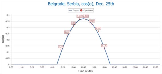
Figure 5. A daylight stack

The experimental points in figure 5 are taken from table 1. The experiment assures the daylight stack theory; the agreement is good if not splendid.

6. High noon observations

Let us now return to our right $\varphi$-triangle indicated on figure 2. Precisely at the noon we hold the triangle ABC in the vertical position, figure 6 left. The hypotenuse $c=\overline{AB}$ traces the direction towards the Polaris. The sun ray, through the vertex A, intersects the horizontal line in the point D, defining the angle $\alpha$ with the opposite $b=\overline{AC}$. The opposite casts the shadow $d=\overline{CD}$, the hypotenuse casts the shadow $a+d=\overline{BD}$. Two light rays, one coming from the Polaris, second coming from the Sun (intersecting each other at the vertex A) by definition define the angle $\gamma$. We infer now from the figure 6 (left) the relation $\left(\gamma -\alpha _{N}\right)+\varphi +\pi /2=\pi$, or

$$\alpha _{\text{N}}=\varphi +\gamma -\pi /2 \tag{10}$$

The letter N stands as the indicator of the true noon moment. This connection of three important angles, at the top of daylight stack, is one of the main consequences of equation (9a).

Now the angle $\gamma$ can be computed as

$$\gamma =\arctan \left(\frac{d}{b}\right)+\pi -\varphi \tag{11}$$

The alternative expression, where the latitude angle is avoided, follows from the cosine law:

$$\cos \gamma =\frac{b^{2}-ad}{c\sqrt{b^{2}+d^{2}}} \tag{12}$$

For example, we registered on January 2^nd^ 2014 ($\tau =11$) in Belgrade, Serbia ($\varphi =44.82^{\circ}N$) $d=41.8$ cm while the height $b=17.6$. From equation (11) $\gamma _{\text{E}}=112.^{\text{o}}2$, and from equation (9b) $\gamma _{\text{T}}=112.^{\text{o}}98$. The error is less than 1%.

As a matter of fact, the angle $\gamma$ varies very little during a few hours before or after the noon — practically, we may determine this angle at any moment near the middle of the given day. Let us see figure 6 (right).

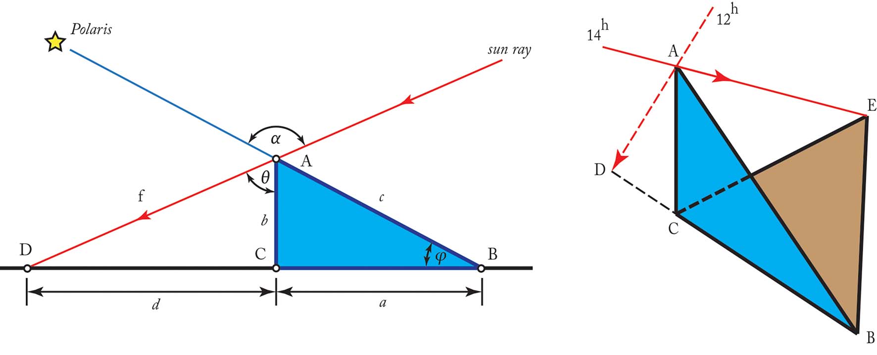
Figure 6. Shadow of right $\varphi -$ triangle, at noon (left) and two hours later (right)

The afternoon shadow of the triangle’s opposite is the length $d_{1}=\overline{CE}$. The shadow of the hypotenuse is $d_{2}=\overline{BE}$. The cosine law now gives

$$\cos \gamma =\frac{b^{2}+c^{2}+d_{1}^{2}-d_{2}^{2}}{2c\sqrt{b^{2}+d_{2}^{2}}} \tag{13}$$

When the Sun is near its zenith, then $d_{1}\to d$, $d_{2}\to d+a$ and the equation (13) takes the form (12), as it should be. Also, we did a small test of the expression (13) in our family manor located in the village of Budimlja, Montenegro ($\varphi =42.86^{\circ}N$), during January 16^th^ 2014 ($\tau =25$). The results are given in table 2.

Time	$d_{1}=CE$[cm]	$d_{2}=BE$[cm]	$\gamma _{E}$[$^{\circ}$]
Local noon	38.5	22.9	110.85
Local noon plus 1h	30.5	45.7	110.10
Local noon plus 2h	38	52.2	110.86
Local noon plus 3h	53	65.6	110.78

Table 2 Measurements of the angle $\gamma$

The mean measured value of $\gamma$ is $110.^{\text{o}}65$, while the corresponding theoretical value, taken from (9b) amounts $111.^{\text{o}}15$.

7. Erastothenian measurement of the year duration

By definition, during days of vernal and autumnal equinoxes, the angle $\gamma$, described by equation (9b) is approaching value of $\pi /2$. Therefore, somewhere around March 21^st^ and September 23^rd^ left side of the equation (9b) can be linearized,

$$\cos \gamma \approx \pi /2-\gamma. \tag{14}$$

Time intervals where this relation holds will be explained later. Now, by serializing cosine part of the right side of the equation (9b) around vernal ($\Omega \tau =\pi /2$) and autumnal ($\Omega \tau =-\pi /2$) equinox points we get

$$\cos \left[\Omega \tau +2e\sin \left(\Omega \tau -\Omega \Delta \tau \right)+2e\sin \left(\Omega \Delta \tau \right)\right]\approx C+D(\Omega \tau \mp \pi /2) \tag{15}$$

where upper ( here ”-”) sign stands for vernal, and lower (here ”+”) sign stands for autumnal equinox (this convention will also hold further through the text), and values of parameters $C$ and $D$ are

$$C=-\sin \left\{2e\left[\cos (\Omega \Delta \tau )\pm \sin (\Omega \Delta \tau )\right]\right\} \tag{16a}$$ $$D=\mp \cos \left(2e\left[\cos (\Omega \Delta \tau )\pm \sin (\Omega \Delta \tau )\right]\right)\left[1\pm 2e\sin (\Omega \Delta \tau )\right] \tag{16b}$$

This linear approximation stands with error no larger than 1% during time intervals from March 1^st^ ($\tau =74$) to April 10^th^ ($\tau =108$) and from September 6^th^ ($\tau =258$) to October 6^th^ ($\tau =288$).

Now, by combining equations (10), (14) and (15), the high noon sun angle $\alpha _{N}$ gets a linear form

$$\alpha _{N}=\varphi \left(C\mp \frac{\pi }{2}D\right)\sin \varepsilon +\left[\Omega D\sin \varepsilon \right]\cdot \tau \tag{17}$$

The rate of change of the angle $\alpha _{N}$ thus should be

$$\frac{d\alpha _{N}}{d\tau }=\Omega D\sin \varepsilon \tag{18}$$

Serializing (16b) around point $\Delta \tau =0$ and exploiting the fact that $2e<<1$ we get

$$\operatorname{D}\approx \mp \left\{\cos \left(2e\right)\pm 2e\left[\cos \left(2e\right)-\sin \left(2e\right)\right]\right\}\Omega \Delta \tau \approx \mp \cos \left(2e\right)\left(1-2e\cdot \Omega \Delta \tau \right), \tag{19}$$

with error no larger than 1% if $\Delta \tau <\left|20\right|$ (that is, if number of days between winter solstice and perihelion is no longer than 20 days).

Combining (18) and (19) we get the quadratic equation

$$\mp 2e\Delta \tau \cdot \Omega ^{2}+\Omega -\frac{1}{\cos \left(2e\right)\cos \varepsilon }\frac{d\alpha _{N}}{d\tau }=0, \tag{20}$$

that has one solution, the orbital angular velocity $\Omega$ as a function of the rate of change of the high noon sun angle $\alpha _{N}$

$$\Omega =\frac{1}{4e\Delta \tau }\left(-1+\sqrt{1\mp \frac{8e\Delta \tau }{\sin \varepsilon \cos \left(2e\right)}\frac{d\alpha _{N}}{d\tau }}\right) \tag{21}$$

We could say that (21) stands for any planet with orbit eccentricity small enough ($2e<<1$), and number of days between winter solstice and perihelion no larger than 20 ($\Delta \tau <\left|20\right|$).

Here we can substitute $\Omega =2\pi /T_{\text{Y}}$. So, the orbital period $T_{\text{Y}}$ of our planet while moving around the Sun is a measurable quantity in the eratosthenian meaning of the word: the equinoctial rate of change of the noon sun angle $\alpha$ tells us how many days takes the Sun to complete one course throughout the zodiac along the ecliptic.

As one can expect from (17), experimental points should lay on the straight line

$$\alpha _{\text{N}}=a\mp b\tau \tag{22}$$

whence we obtain $d\alpha _{\text{N}}/d\tau =\mp b$. Let us insert this experimental datum into (21). Finally, solving (21) for the period $T_{\text{Y}}$ we get

$$T_{\text{Y}}=360^{\text{o}}\cdot \frac{4e\Delta \tau }{-1+\sqrt{1+\frac{8e\Delta \tau b}{\sin \varepsilon \cos \left(2e\right)}}} \tag{23}$$

This is our formula for experimental assessment of the year’s length by measuring noon sun angle around equinoxes. If the approximation $\frac{8e\Delta \tau b}{\sin \varepsilon \cos \left(2e\right)}<<1$ is valid, we are reaching the simplified form

$$T_{\text{Y}}=\frac{360^{\text{o}}\sin \varepsilon \cos \left(2e\right)}{b} \tag{24}$$

In our epoch, on the Earth $\varepsilon =23.4^{\circ}$ and $e=0.0167$, hence the “lightweight” formula suitable for measurements on the Earth is

$$T_{\text{Y}}=\frac{143}{b} \tag{25}$$

This formula says that once the coefficient $b$ (measured in degrees per day) is known, the number of days in the year is readily obtainable.

We have experimentally scrutinized the new formula (23) during early spring in 2014, which was full of clear days. We have recorded the high noon shadows in Belgrade, Serbia by means of our right $\varphi -$ triangle, from February $4^{\text{th}}$ to April $19^{\text{th}}$ 2014. The experimental data are shown on figure 8 as points, together with the full line which represents the noon sun angle plotted against days of year. As we estimated, the true linear section of the curve goes from March 1^st^ to March 26^th^. The data which belong to this period are given in table 3.

Belgrade, Serbia ($\varphi =44.82^{\circ}N$)
Gregorian date	01.03	09.03	12.03	13.03	14.03	26.03
Eratosthenian date	69	77	80	81	82	94
Alpha ($^{\circ}$)	52,4	49,27	48,13	47,78	47,33	42,6

Table 3. Measurements of the noon sun angle in Belgrade, Serbia during spring 2014.

The best fit for these six points is found to be the line $\alpha _{\text{N}}=a-b\tau$ with $a=79.4648$ degrees and $b=0.39188$ degrees per day.

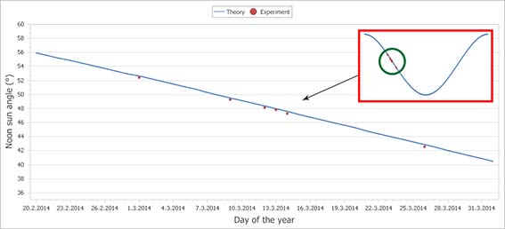
Figure 7. Experimental points on the vernal descent of the noon sun angle curve. The full year curve is shown in the upper right corner.

So we get the value for $b$ which is necessary for the evaluation of the year duration. Inserting this experimental datum into (19) we find

$$T_{\text{Y}}=\frac{143}{0.39188}=364.9\;\text{days} \tag{26}$$

To be sure, this was a successful attempt. The result seems quite good. Nevertheless, reaching the error of only $0.1\%$ we didn’t found us in a state of triumphant exaltation: maybe we did this job under the influence of a lucky star (as once did Eratosthenes himself reaching the exceptionally accurate result for the circumference of the Earth). Anyway, we see formula (23) as a personal homage to the Eratosthenes and his unique scientific attainment.

9. Conclusion

The exceptional work and personality of great Eratosthenes was the basis inspiration for this paper, its notions and results. His measurement of the Earth’s circumference, associated with some results of Archimedes, extends the whole history of physics to more than two millenniums. Anytime we are aware of our own shadow at a clear day, we are astounded with the fact that the Sun not only lightens us but in addition enlightens us: sun rays supply us with a wide range of physical ideas — from geometry, via kinematic to thermodynamics and optics.

The beauty and efficiency of the eratosthenian way of thinking motivated us to incorporate the shadow length measurement method into a university course of environmental physics.

We searched for a suitable mathematical model for the irradiation of a globe in the vicinity of a point source of light and we believe that such a model is quite well represented by equations (9). We successfully tested the predicted sun angle by a fairly simple tool, the tripod type gnomon.

Also, we derived a simple formula (25) suitable for the Eratosthenian measurements of year duration. This formula is, as we believe, a new result. We proved it experimentally by the high noon shadow length measurements during merely several days of March.

Appendix: The day marshal Kaine got married

Eratosthenes’ approach in solving problems by measuring shadow length actually stretches beyond science and university education. As an amusing example we shall now find, using equations (9) and (10), the date when marshal Will Kaine, hero of the Hollywood movie High Noon³ (1952), brilliantly presented by Gary Cooper, got married.

Briefly speaking, marshal Kaine decided to retire from his service in the (imaginary) town of Hadleyville. He just got married when the group of bandits came to terrorize citizens. Kaine in vain tried to get help for facing the menace. Therefore, in the famous scene presented on figure A, Kaine stands alone on the empty street.

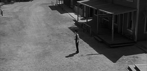
Figure A. A man is always accompanied by his shadow and destiny: Kaine’s solitude

Carefully measuring the length of Kaine’s shadow, we found that at this moment, which movie itself defined as the high noon, our sun angle equals $\alpha =27.47^{\circ}$. A brief Internet search gave us a couple of important information: latitude of the filming location was $\varphi =34.15^{\circ}N$ and the filming was conducted in the late summer and early autumn. Also, the film suggests through series of clues such as the calendar on the wall and the newspapers’ headlines that the year in which story took place was 1898.

Equation (10) gives us the value of the daily angle:

$$\gamma =\alpha -\varphi +90^{\circ}=83.32^{\circ} \tag{A1}$$

Solving equation (9b) for $\tau$ gives two solutions, Eratosthean dates, $\tau =106$ and $\tau =256$, which correspond to Gregorian dates April 7^th^ and September 6^th^, respectively. We can conclude that scene from Figure A represents exactly Sunday, September 4^th^ 1898.

References

[1] See the article: The most beautiful experiment, Physics World, Sept. 1, 2002.

[2] Gubelkian, E. (1987) The Origin and Value of the Stadion Unit used by Eratosthenes in the Third Century BC, Archiv for History and Sciences, (4)37; p. 359.

[3] V M Babović and S Mekić, The Bravais Pendulum: The Distinct Charm Of An Almost Forgotten Experiment, Eur. J. Phys. 32 (2011) 1077-1086.

[4] Miloš Babović and Vukota Babović, How Needless Are Buffon’s Needles? Eur. J. Phys. 34 (2013) 715-728.

[5] Carroll, J and Hughes, S (1913) Using a video camera to measure the radius of the earth, Physics education 48: 731.

[6] A.V.Bjalko, Our Planet — Earth (in russian), Science, Moscow 1983

[7] Karttunen, H. et al (2007) Fundamental Astronomy, Fifth Ed, Springer-Verlag, Heidelberg; p. 115.

[8] Danby, J. M. (1988) Fundamentals of Celestial Mechanics, 2nd ed., Willmann-Bell, p. 200.

[9] (2002), Philip’s Astronomy Encyclopedia, Philip’s.

[10] United States Naval Observatory, 1992. The astronomical almanac for the year 1992. US Government Printing Office.

[11] W.C.Forsythe, E.J.Rykiel Jr, R.S.Stahl, H.Wu, R.M.Schoolfield, A model comparison for daylength as a function of latitude and day of year, Ecological Modeling 80 (1995)87-95.

[12] Khavrus V, and Shelevytsky I, (2010) Introduction to solar motion geometry on the basis of a simple model, Physics Eduacation, 45(6): 641.

[13] Khavrus V, and Shelevytsky I, (2012) Geometry and the physics of seasons, Physics Education, 47(6): 680.

[14] Vorontsov-Vel’yaminov, BA. (1969) Astronomical Problems, Pergamon Press, Oxford; p.46.

Footnotes

1. We had a head-start advantage since our measurements took place in Belgrade, Serbia: manual creation of such a tool was not necessary. Namely, the latitude of Belgrade, Serbia is almost precisely 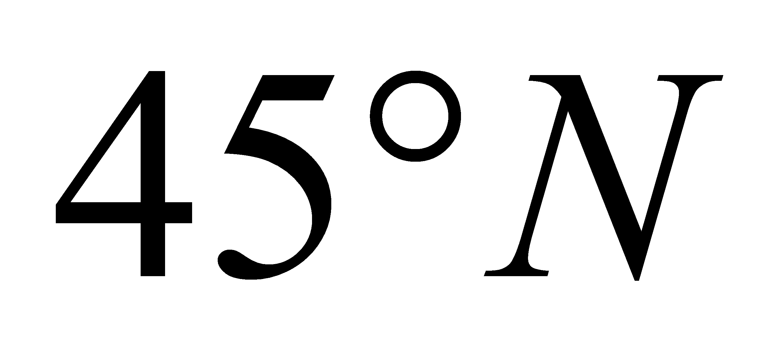, so everyone in our city (just like those living in places with latitudes 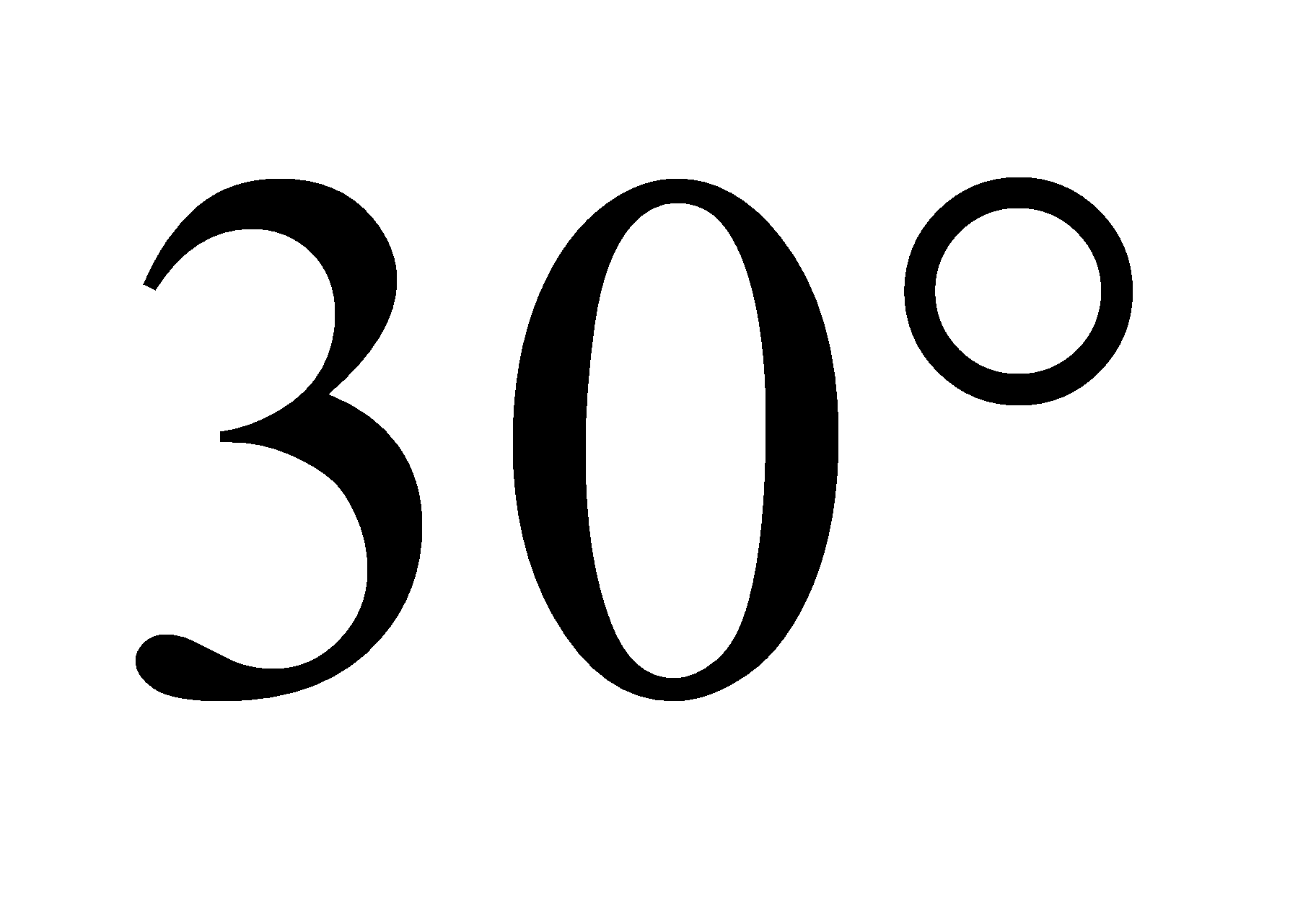or 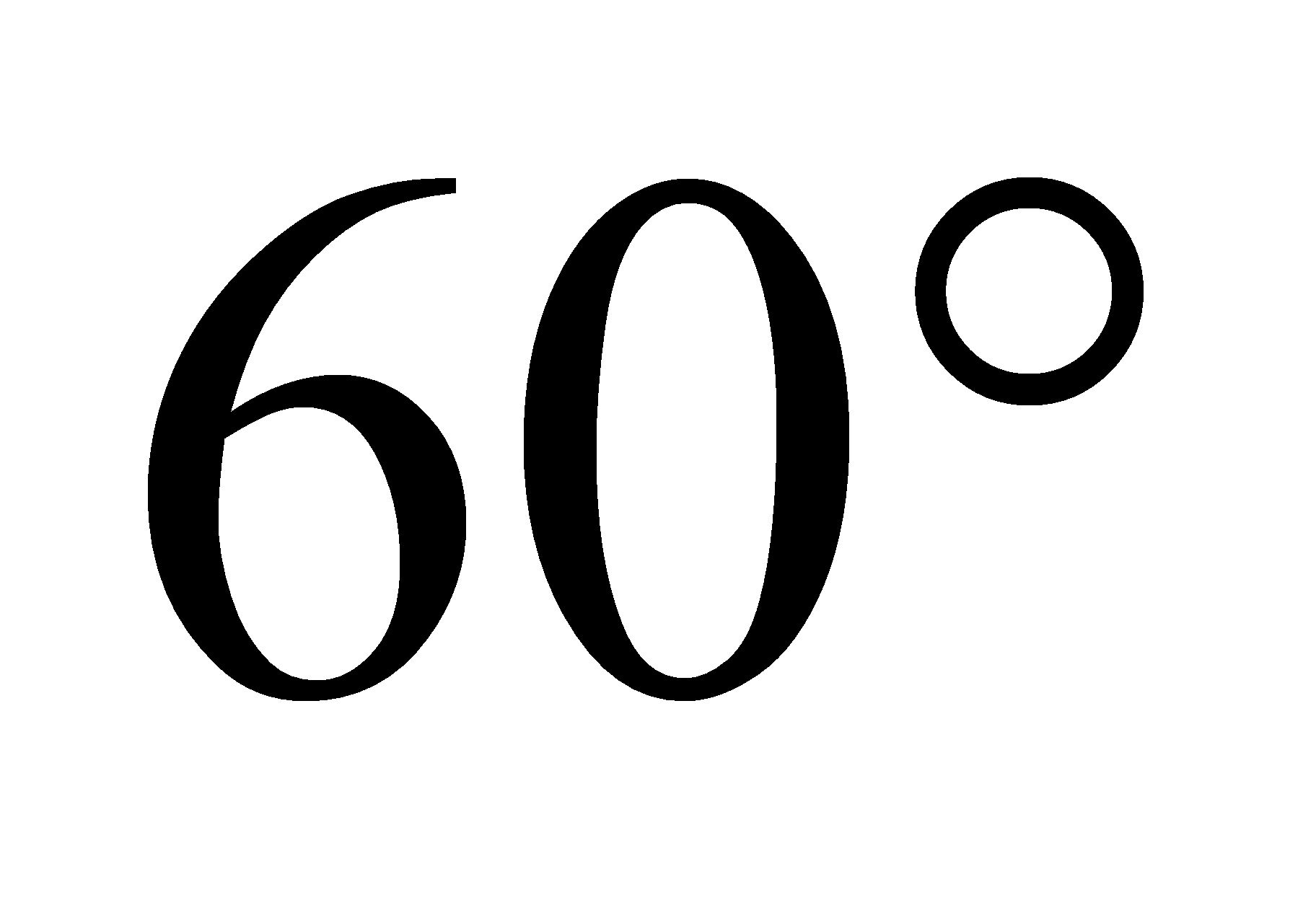north or south) can purchase a right $\varphi -$ triangle in a supermarket. ↩

2. Western civilization named two types of the calendar year after rulers, secular or religious, and none after a person from the science. We propose the name Eratosthenes’ year for the calendar year that starts on December 23^rd^ according to the Gregorian calendar. ↩

3. http://www.imdb.com/title/tt0044706/ ↩