The magnetic force on a thin ferromagnetic cylinder inside a permanent U-shaped magnet: Modeling the phenomenon

Miloš Babović$^{1}$ and Vukota Babović$^{2}$

1 Pariske komune 63, New Belgrade, Serbia

2 Piva Karamatijeviá 29, Belgrade, Serbia

E-mail: milos.babovic@gmail.com and bvukot@sezampro.rs

Abstract

Recently we have described an original experiment with a U-shaped permanent magnet [7]. Oscillations of a thin ferromagnetic cylinder can arise inside the magnet. In the current paper we analyze these oscillations. While the experiment is simple and amusing, the theory of phenomenon is not quite elementary. We have succeeded in searching for the true restoring force; although approximate, our formula turns to be effective. The numerical solution of the equation of oscillations has been successfully compared with experimental data. The involved heuristic possibilities have been briefly commented. We believe the experiment is useful for students, because it can help the right comprehension of a general formula for magnetic force.

1. Introduction

The concept of the force acting on a small fixed charged sphere in an external electrostatic field, i.e. $\vec{F}=q\vec{E}$, hardly causes misunderstandings among students. The mathematics required is not very demanding and computations are almost direct. For an example, a small sphere is quit a good model for a charged water droplet. There are in nature physical objects such as electrons and protons; we all encourage students, at list in the beginning of their physics education, to conceive these particles as spheres that attract or repel one another and interact with external fields.

However, the definition of magnetic force acting on a body in an external magnetostatic field may appear a little odd to many of students. The reason is evident: the magnetic monopole, a hypothetical elementary particle with only one magnetic pole, does not exist in nature. Instead we must deal with forces on moving electric charges, or often in practice on current carrying wires, $\Delta \vec{F}=I\left(\Delta \vec{l}\times \vec{B}\right)$. Evidently, some knowledge of vector analyses is required [B]. The very concept of a short, (mentally) isolated, current carrying element $I\Delta \vec{l}$, which plays the basic role in the law which governs the forces acting on currents in a magnetic field, turns to be a problem an sich [A]. The geometry of currents and inhomogeneity of external fields can bring other conceptual and computational complications [1].

Therefore, every simple experiment which can help students in deepening their understanding of magnetic force is welcome. In this article we are going to explain pin oscillations inside a U-shaped permanent magnet. We believe this is an experiment of that sort. Being simple to perform, the experiment is rich as a phenomenon. The inclusion of knowledges from various branches in physics (kinematics, dynamics, magnetism) is necessary for the explanation. This multidisciplinary approach may appear as an advantage if students tend to integrate their isolate skills accomplished in various courses.

Let us at the beginning recall some of basic formulas. It would assist the reader with his comfortable paper reading.

2. Short comment on magnetic force

The force $d\vec{F}$ acting on an elementary segment $d\vec{l}$ of some wire loop currying stationary current I in an external magnetic field of an induction $\vec{B}$ is governed by the law [2]

$$d\vec{F}=I\left(d\vec{l}\times \vec{B}\right). \tag{1}$$

The resultant Ampѐre’s force acting on a current loop is given by the circulation of the magnetic induction along the closed path coincidental with the loop:

$$\vec{F}=I\oint \left(d\vec{l}\times \vec{B}\right). \tag{2}$$

According to this expression the resultant force is zero if the field is everywhere homogenous ($\vec{B}=\text{const}$).

Let us assume that a plane current loop is sufficiently small (elementary current loop). It bounds a very small surface $dS$. Such a loop can be conveniently characterized by its magnetic moment

$$\vec{p}_{\text{m}}=IdS\;\vec{n}=p_{\text{m}}\;\vec{n}. \tag{3}$$

Here $\vec{n}$ represent the unit vector of the surface perpendicular (the direction of $\vec{n}$ is connected with the direction of the current in the loop through the right-hand screw rule). Starting from the expression (2) we can get the general expression for the force acting on an elementary current loop in a nonuniform magnetic field [3]:

$$\vec{F}=p_{\text{m}}\frac{\partial \vec{B}}{\partial n}. \tag{4}$$

Here $p_{\text{m}}$ stands for the magnitude of the magnetic moment of the loop. The derivative of vector $\vec{B}$ must be taken along the normal, i.e. along the direction of vector $\vec{p}_{\text{m}}$. So, the direction of force is neither the direction of the magnetic moment nor the direction of the magnetic induction; the force is along the direction of the elementary increment of vector $\vec{B}$. Students may deepen their understanding of this important point analyzing the fallowing example.

A thin and long, strait conductor is placed along the z axis (figure 1). An elementary current loop lies in the $\left(x,z\right)$ plane; its vector $\vec{p}_{\text{m}}$ points along the y axis. A force arises which tends to pull the loop towards the conductor, figure 1 (left). What is the reason, according to formula (4)?

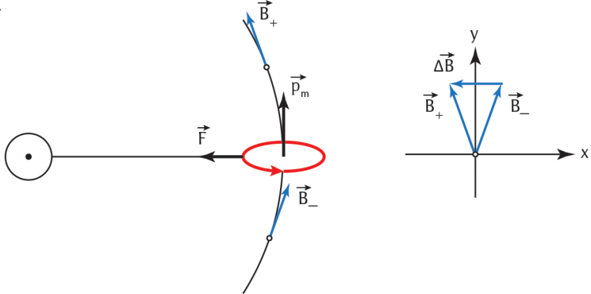
Figure 1. Left: current loop near strait conductor. Right: induction increment

The induction vector just below the loop is $\vec{B}_{-}$, and just above it $\vec{B}_{+}$. The induction increment vector, along the direction of the magnetic moment, is caused only by the change of the direction of the vector $\vec{B}$ and equals $\Delta \vec{B}=\vec{B}_{+}-\vec{B}_{-}$ (figure 1, right). Really, the increment, thereby the force, sees toward the origin. Basically, the involved mathematics is almost the same as in the case of a uniform circular motion of a material point, when one analyses the centripetal acceleration. Therefore we can conclude (After Feynman who spoke: the same equations have the same solutions [4])

$$F=p_{\text{m}}\frac{B}{r}. \tag{5}$$

Here $B=\mu _{0}I/\left(2\pi r\right)$ is the magnitude of the induction at a locus with distance $r$ from the conductor [5].

Assume the current loop is momentarily at rest at some point $x=-a$. The force (5) pulls the current loop causing it to slide on right, toward the conductor. But if the starting point is at $x=+a$, the effect would be the same: the loop slides on left toward the conductor. Nevertheless, the loop cannot oscillate along the $x$ axis, even in a fairytale-case of fantastic, quite passable door at the conductor. Simply, the field is singular at the origin. This magnetic ”black hole” will ”absorb ” the loop.

If only we could get a magnetic field with field lines (nearly) circular, but giving enough strong force on a loop at $x=\pm a$ and zero or feeble force in the center! The confiner of such profile might be good scenery to maintain the magnetic dipole oscillations. Remark that in (5) $F\propto 1/r^{2}$, whereas the inverse proportionality $F\propto r^{2}$ would do the job.

Not without a surprise we have realized that such a magnetic field configuration is within our touch. That is what we shall henceforth talk about.

3. U-shaped magnet with a glass guide attached

Figure 2 shows field lines of a classical U-shaped magnet. Concentrate our attention on the space between the magnet poles. We see one straight line connecting the north pole (blue) with the south pole (red). Left and right from this line lay lines which are concave and convex curves, respectively. The central part of this picture gives a rude resemblance to the sketch of field lines in the vicinity of a straight current conductor, but with one important difference: the line curvature grows with the distance (left or right the same) from the strait line. And this magnetic field is right what we sought. That an elementary current loop would oscillate inside a U-shaped magnet seems now a reasonable expectation.

Figure 2. U-shaped magnet: sketch of force lines

Well, the fabrication of a small current loop may appear a complicate job. Why, we can avoid this annoyance. We shall place inside the magnet an iron pin instead of the loop. By the magnetisation the pin would transform into a thin bar magnet having a induced magnetic moment $\vec{\mu}$. A bar magnet is equivalent to a cylindrical solenoidal current [6] having the same magnetic moment, $\vec{p}_{\text{m}}=\vec{\mu}$. Hence we can say much about the force upon the pin using the general formula (4).

Our magnet is a U-shaped piece (90 mm long, 25 mm in width, 7 mm thick; hands 47 mm apart) taken from a standard classroom kit.

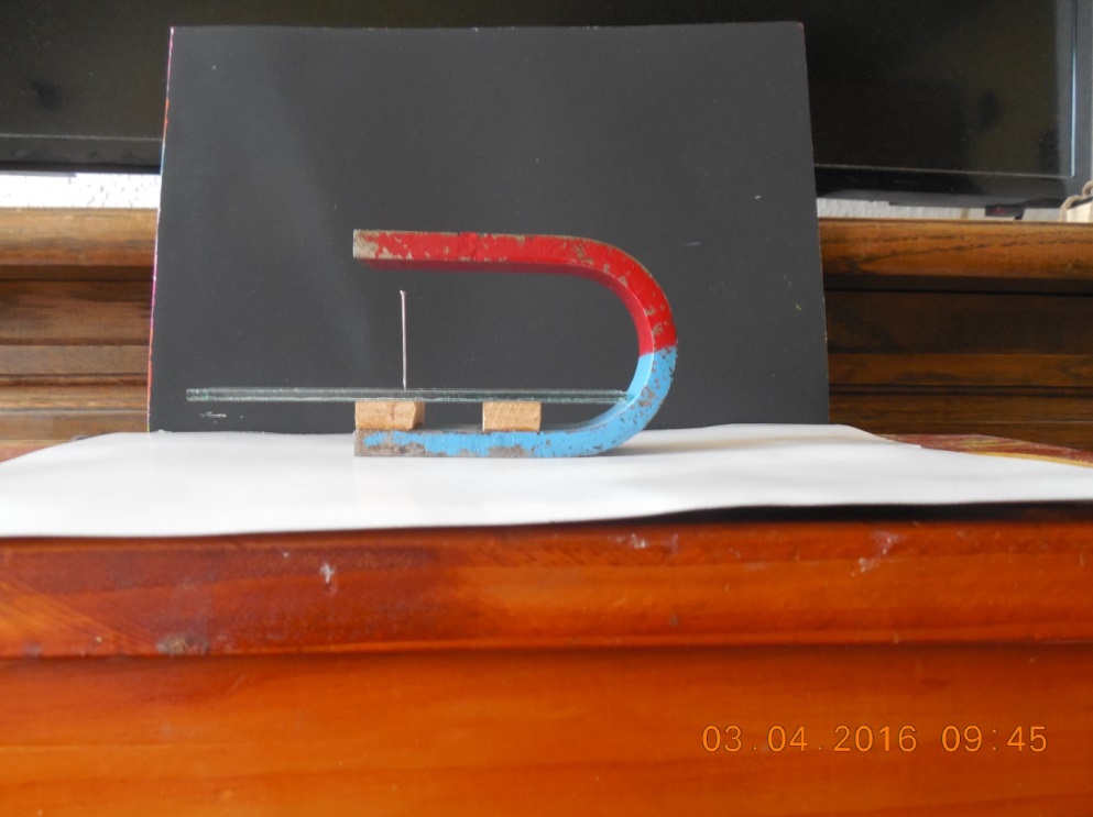
Figure 3. Guide for pin sliding

To support (almost) friction-less motion of a pin, with its center of mass always laying in the plane of symmetry, we mount a guide on two wooden supports, as shown on figure 3. The guide is made as the glass plate 2 mm thick and 125 mm long. The 45 mm long guide piece stretches outside the magnet. (The pin shown is at rest in its equilibrium position.) More technical details may be found in [7].

Now we shall describe our experiments on guided pin oscillations in the magnetic field of the U-shaped magnet.

4. Experiments. Collecting pin motion data

The pin released from certain point in the interior of the magnet slides along the guide. It arrives the equilibrium point but continue to slide outward the magnet until it riches the first turning point. Thereafter the pin moves back — the oscillations around the equilibrium point arise. The oscillations are damped and the pin stops after several cycles.

This pin oscillation experiment can be easily performed. The repetition of measurements makes no problems; taking one or other place for the starting point, one can in short time collect data which represent a set of points {time, position}. One full oscillatory cycle is over but in few seconds.

Our observing and registering technique is based on taking video clips, which record the kinematic details during the pin motion. A video clip is sequence of successive photos (each of which is usually termed as a frame).

We used a Nikon L610 camera which can match these requests. Recording with Nikon L610 an event which covers one second in real time means that we have a full HD PAL video (25 fps) lasting two seconds (50/25=2). (Nota bene: We regret that we have been lacking any of new camera models which can capture up to 1000 fps [8], for recording oscillations in small-amplitude regions.)

The moments in which the oscillating pin reaches consecutive turning points can be read off from the corresponding video. The procedure demands to examine the video as the sequence of frames. The zero instant refers to the first frame in which we see that the pin starts. The second frame is taken after the time interval $\Delta t_{50}=1/50=0.02$ seconds, and so on. In that way we define the discrete time coordinate. The successive amplitude positions, the pin turnpoints, were marked by a vertical line on each of corresponding frames. So we have been able to collect the set of points $\left\{\text{time},\text{position}\right\}$ from a particular video. An example will be given in section 6, where we also intend to compare the experiment with theory.

We shall now try to give a physical picture adequate for this oscillating phenomenon.

5. Restoring force. Semi-theoretical approach

Let us assume the mass center of the pin moves along the x axis (symmetry axis), as sketched in figure 4. The motion starts at some point $x=0$ (the origin) inside the magnet. The equilibrium point is at $x=x_{\text{E}}$. An auxiliary coordinate $\xi$ may be introduced via the relation $\xi =x-x_{\text{E}}$; the $\xi$ measures pin displacement from the equilibrium position. The outward direction is for positive displacements.

Figure 4. Magnet geometry; measures and symmetry axis

The pin motion law $\xi \left(t\right)$ follows from the solution of the differential equation

$$M\frac{d^{2}\xi }{dt^{2}}=-F\left(\xi \right)+\text{friction}. \tag{6}$$

We represent a vertically oriented pin with a point mas $M$ moving along the $\xi$ axis. Here $F\left(\xi \right)$ is the magnetic force which acts on a pin; for the force we will apply the formula (5). The force is directed towards the equilibrium point, always opposing the displacement. In passing, let us remark that we have also sought for the force expression using the formal theory of magnetism, in which one takes there are fictive magnetic charges $\pm m$ on the pin ends. In this conception the pin emerged into a magnetic field becomes a magnetic dipole having a certain magnetic moment $\mu$. It is very well that this rude theory gives the relationship which coincides with the formula (5). The proof is simple and may be found in [7].

Well, we don’t know what might be the exact expression for $F\left(\xi \right)$, although we have the formula (5). Simply, we are lack for the entire data set defining the pin-magnet physical system. In the first place, the function $B\left(\xi \right)$ is unknown. Second, the curvature of a field line determines the force in a crucial way and we don’t know how in detail. We must try to overcome these difficulties.

Let us proceed as follows.

Figure 5 shows a field line inside the magnet. Our idea is to approximate this line with a half of an ellipse. (Watching on details in figure 2 we may learn that minor disagreements can arise only far from the plane of symmetry, in regions which are unimportant for the defining of force.)

The center of this ellipse lies in the equilibrium point $\text{E}$. The major axis $a$ equals the segment $\text{ET}$, the point T being the ellipse vertex. The field line of length $2b$, which connects the two magnet arms passing through the point $\text{E}$ is the ellipse double minor axis. The focus is denoted with $\text{Z}$. The perpendicular $\ell$ stands for the semi-latus rectum.

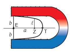
Figure 5. Approximating field line with an ellipse (Slika!)

We need the expression $k$ for the ellipse curvature. This well-known formula reads [9]

$$k=\frac{1}{a^{2}b^{2}}\left(\frac{x^{2}}{a^{4}}+\frac{y^{2}}{b^{4}}\right)^{-3/2}. \tag{7}$$

The curvature in the vertex follows for $y=0$ and $x=a$. Hence the result is

$$k=\frac{a}{b^{2}}=\frac{1}{\ell }. \tag{8}$$

Our expression for the magnetic force (5) can be now rewritten in the form

$$F=p_{\text{m}}Bk, \tag{9}$$

because the radius $r$ is the reciprocal of the curvature $k$. Let us observe that the major axis may be in (8) replaced with the displacement coordinate, i. e. put $a=\xi$. The minor axis is here simply a constant of the magnet, $b=2.2$ cm in our set-up.

Hence we can put equ. (4) into the form

$$F=F_{0}\beta \left(\xi /b\right)\frac{\xi }{b}. \tag{10}$$

The induction depends on displacement and we have inserted here $B=B_{\text{E}}\beta \left(\xi /b\right)$, with $B_{\text{E}}$ for the induction in the point E. So we get a constant factor $F_{0}=p_{\text{m}}B_{\text{E}}/b$. Let us expand the function $\beta \left(\xi /b\right)$:

$$\beta \left(\xi /b\right)=1+c_{1}\frac{\xi }{b}+c_{2}\left(\frac{\xi }{b}\right)^{2}+... \tag{11}$$

Therefore, the magnetic force appears to be

$$F=F_{0}\left(\zeta +c_{1}\zeta ^{2}+c_{2}\zeta ^{3}+...\right). \tag{12}$$

We have introduced the normalized coordinate $\zeta =\xi /b$. The two dimensionless constants $c_{1}$ and $c_{2}$ shall be discussed later.

6. Physical model of the phenomenon. Numerical treatment

According to the above elaborated assumptions let us transform and modify the pin motion equation as follows:

$$\frac{d^{2}\zeta }{dt^{2}}+\Omega ^{2}\left(\zeta +c_{1}\zeta ^{2}+c_{2}\zeta ^{3}\right)+\left[\gamma _{1}d\zeta /dt+\gamma _{2}\left(d\zeta /dt\right)^{2}\right]=0. \tag{13}$$

We have introduce the parameter $\Omega$ according to the relation

$$\Omega ^{2}=F_{0}/Mb. \tag{14}$$

In the case of frictionless oscillation just in the vicinity of the equilibrium point (small displacements) the equation (13) reduces to $\ddot{\zeta}+\Omega ^{2}\zeta \simeq 0$, i. e. gives simple harmonic solutions. The experiment maintains this conclusion. The nonlinear effects start to play an important role for $\zeta \sim c_{1}^{-1}$ (roughly speaking, as we shall see, for displacements exceeding 3 cm).

However, some amount of friction must be added in (13) and we did it. In fact, at least three types of friction could be involved in pin motion. First, kinetic friction for surfaces in relative motion (pin sliding against glass surface), second, air resistance (pin of given size and shape moving with respect to air of given parameters), and third, eddy currents in metal body oscillating in external magnetic field. Therefore we have allowed that the whole frictional force is proportional to the velocity (the coefficient $\gamma _{1}$) as well as to the squared velocity (the coefficient $\gamma _{2}$) of the pin. The two terms are indicated inside the square brackets. Our model of the phenomenon (in the sense elucidated in [10]) is now completed.

Accordingly we have a nonlinear, ordinary differential equation of the second order, where the normalized coordinate $\zeta$ is an unknown function of time. The equation is rather complex and we must try to solve it numerically. But how can we guess what may be the parameters with which we should start the solving process? The abscissae of the points $A_{3}$ and $A_{5}$ are $t_{3}=0.3$ s and $t_{5}=0.56$ s (see below the experimental data). Hence the corresponding time interval is $T=0.26$ s. Therefore we guess $\Omega =2\pi /T\simeq 24\,\text{s}^{-1}$, i. e. $\Omega ^{2}\simeq 576\,\text{s}^{-2}$. Also we have retained here the proportion $1:0.58:0.13$, established experimentally and presented in figure 5 of the paper [4,]. For the sake of some minor corrections we have varied constants $\gamma _{1}$ and $\gamma _{2}$ trying to achieve the agreement with the experiment as good as possible.

Well, let us conclude. We have found that the set of parameters $\Omega ^{2}=576\,\text{s}^{-2}$, $c_{1}=-0.58$, $c_{2}=0.13$, as well as $\gamma _{1}=2.8\,\text{s}^{-1}$ and $\gamma _{2}=0.86$ are preferable for fitting the experimental data.

The full line on figure 5 plots the numerical solution of equation (13). The full points on the same figure represent the experimental data (collected as explained in section 4)

$\left\{t,\zeta \right\}\equiv$ $\{\{ 0,0.73\},\{ 0.16, - 1.29\},\{ 0.3,0.52\},\{ 0.42, - 0.79\},\{ 0.56,0.41\},\{ 0.68, - 0.41\},\{ 0.78,0.2\},\{ 0.9, - 0.16\}\}$.

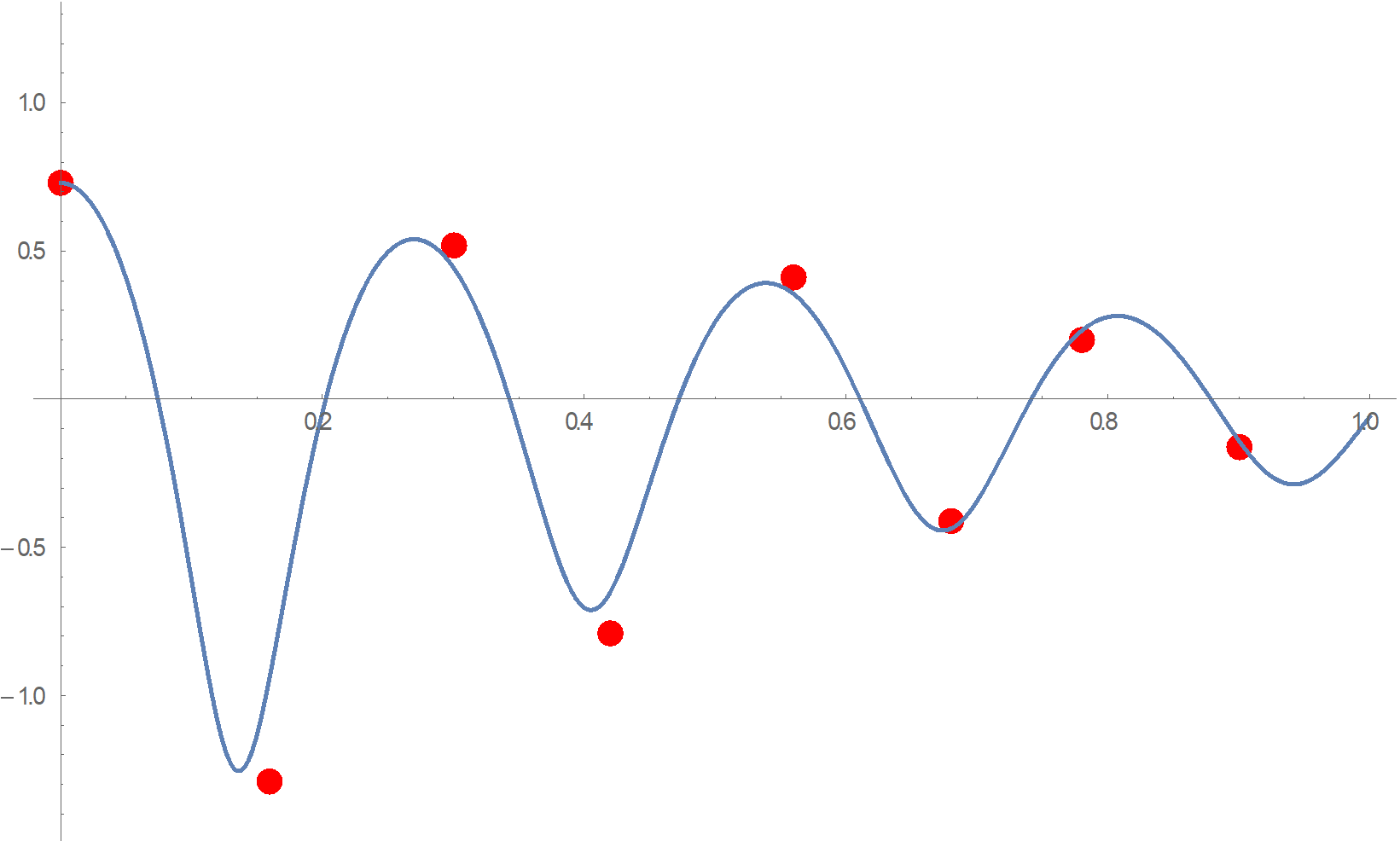
Figure 5. Experimental points and computed oscillating curve

The agreement between theory and experiment seems satisfactory. In particular, the curve passes closely the turnpoints $A_{2}\left(0.16,-1.29\right)$ and $A_{3}\left(0.3,0.52\right)$, which is unattainable in the simple harmonic motion approximation. The reader can more learn about the agreement studying the percentages presented in the table below.

Table. The experiment vs. computation comparison of the turnpoints

	$A_{1}$	$A_{2}$	$A_{3}$	$A_{4}$	$A_{5}$	$A_{6}$	$A_{7}$	$A_{8}$
$\delta t\left[\%\right]$	0	15.5	9.27	3.28	3.47	8.23	3.56	4.62
$\delta a\left[\%\right]$	0	2.56	5.9	9.3	4.46	10.6	43.6	85.12

The two rows show the abscissa and ordinate differences for corresponding maxima. For instance, we read for the turnpoint $A_{4}$: $\left|t_{\text{theor}}-t_{\exp }\right|/t_{\exp }=3.28\%$ and $\left|a_{\text{theor}}-a_{\exp }\right|/a_{\exp }=9.3\%$. The deviation $\delta a=43.6\left[\%\right]$ for $A_{7}$, as well as $\delta a=85.12\left[\%\right]$ for $A_{8}$ of cause are not so negligible; but we have expected these results: the uncertainty of readouts for small amplitudes was appreciable in our measurements (fine quantum equipment - 100 or more frames per second - would be desirable) [7].

From the equation (14) one may easily obtain the relation $~p_{\text{m}}B_{\text{E}}=Mb^{2}\Omega ^{2}$. The quantities on the right hand side are now all known. The computations give

$~p_{\text{m}}B_{\text{E}}=3\cdot 10^{-7}$ Nm. (15)

Suppose we have somehow learned the induction at the equilibrium point; let us denote this figure in SI as $B_{\text{E}}\left[\text{T}\right]$. If so, it follows from equation (14)

$$~p_{\text{m}}=\frac{3}{B_{\text{E}}\left[T\right]}\cdot 10^{-7}\,\text{Am}^{2} \tag{16}$$

Dynamical measurements of the type described allow us to evaluate the magnetic moment (comp. [11]) of a ferromagnetic pin once the basic intrinsic parameters of the U-shaped magnet are known.

7. Conclusion

It seems that new generations of permanent magnets tend to displace classical magnets from lab kits [12], [13]. We don’t think that U-shaped magnets are now but a museum piece. Working with them we concluded that they are very suitable for both undergraduate and graduate experiments on oscillating motions. In this paper we show that these experiments are simple, impressive and easy to repeat (the features that are always respectable [14]). At the same time, they have an appreciable heuristic and educating potential. Schoolboys find them amusing. For students they might be a call toward deeper understanding of magnetic forces, oscillating motions and nonlinear dynamical effects. Both simple and modern, these classroom measurements call for analytical as well as computer-supported numerical explanations.

References

[1] C A Manogue et al. (2006) Why is Amperes law so hard? A look at middle-division physics, Am J Phys 74(4), p. 344.

[2] Halliday and Resnick, Fundamentals of Physics, third edition, John Wiley & Sons, Inc. 1988; p 700.

[3] I E Irodov, Basic laws of electromagnetism, Mir Publishers, Moscow 1986; p. 158, equ. 6.33.

[4] R P Feynman et al, The Feynman Lectures on Physics, Vol. II, Addison-Wesley Publ. Comp, Inc, London 1963; Ch. 12: Electrostatic Analogues.

[5] R.A.Serway,Principles of Physics, second edition, Saunders College Publishing, London 1994; p. 649, eq. [22.14].

[6] I E Tamm, Fundamentals of the Theory of Electricity, Mir Publishers, Moscow 1979; p. 310: “From the viewpoint of the electron theory, a magnet is equivalent to a cylindrical solenoidal current”.

[7] Miloš Babović and Vukota Babović, A few simple classroom experiments with a permanent U-shaped magnet, Physics Education, 52(1).

[8] Andre Heck and Peter Uylings (2010) In a hurry to work with high-speed video at school, The Physics Teacher 48(3), pp. 176-181.

[9] https://en.wikipedia.org/wiki/Ellipse

[10] Christine Waltner et al (2011) How iron becomes magnetized — the introduction of a model of ferromagnetism in secondary school physics, Phys Educ 46(3), p. 259.

[11] KM Najiya Maryam (2014) EM induction experiment to determine the moment of a magnet, Physics Education, 49(3), p. 319.

[12] Deborach Wood and John Sebranek, Electromagnetic Induction with Neodymium Magnets, TPT Vol 51, Sept 2013, pp. 344-345.

[13] Gerald Feldman, Dramatic (and Simple!) Demonstration of Newton’s Third Law, TPT Vol 49, Feb 2011, pp. 103-105.

[14] Kerry Browne and David P. Jackson, Simple Experiments to Help Students Understand Magnetic Phenomena, The Physics Theacher, Vol 45, Oct 2007, pp. 425 — 429.

[15] https://www.youtube.com/watch?v=tWFE2RZW-uQ

[A] Jackson, p. 189 (214)

[B] Stratton